

Table of Contents
- Introduction
- Setup
- Ibis: Compile Once, Run Anywhere
- Narwhals: The Zero-Dependency Compatibility Layer
- Fugue: Keep Your Code, Swap the Engine
- Summary
Introduction
The backend you start with is not always the backend you finish with. Teams commonly prototype in pandas, scale in Spark, or transition from DuckDB to a warehouse environment. Maintaining separate implementations of the same pipeline across backends can quickly become costly and error-prone.
Rather than reimplementing the same pipeline, you can define the logic once and execute it on different backends with one of these tools:
- Ibis: Uses its own expression API and compiles it to backend-native SQL. Best for data scientists working across SQL systems.
- Narwhals: Exposes a Polars-like API on top of the user’s existing dataframe library. Best for library authors building dataframe-agnostic tools.
- Fugue: Runs Python functions and FugueSQL across distributed engines. Best for data engineers scaling pandas workflows to Spark, Dask, or Ray.
In this article, we’ll walk through these three tools side by side so you can choose the portability approach that best fits your workflow.
💻 Get the Code: The complete source code and Jupyter notebook for this tutorial are available on GitHub. Clone it to follow along!
Setup
All examples in this article use the NYC Yellow Taxi dataset (January 2024, ~3M rows). Download the Parquet file before getting started:
curl -O https://d37ci6vzurychx.cloudfront.net/trip-data/yellow_tripdata_2024-01.parquet
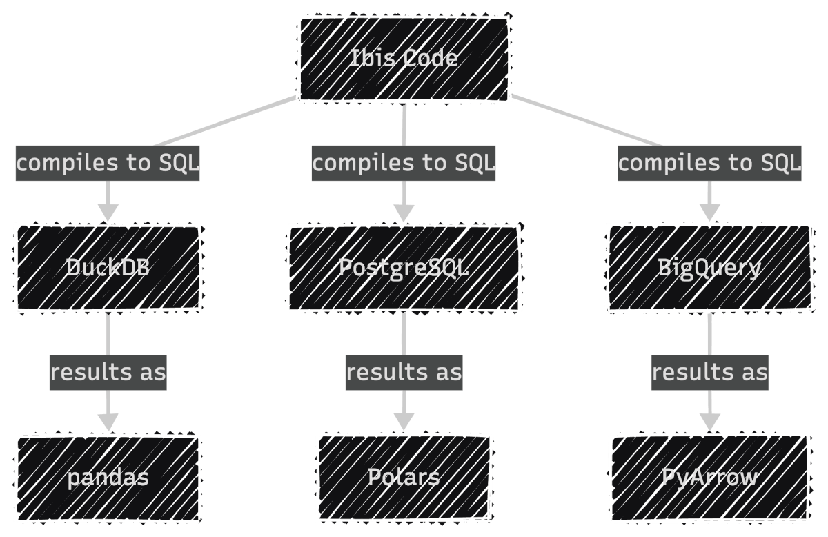
Ibis: Compile Once, Run Anywhere
Ibis provides a declarative Python API that compiles to SQL:
- What it does: Translates Python expressions into backend-native SQL for DuckDB, PostgreSQL, BigQuery, Snowflake, and 22+ other backends
- How it works: Compiles expressions to SQL and delegates execution to the backend engine
- Who it’s for: Data scientists working across SQL systems who want one API for all backends
In other words, Ibis compiles your code to SQL for the backend, then lets you collect results as pandas, Polars, or PyArrow:
To get started, install Ibis with the DuckDB backend since DuckDB is fast and needs no server setup:
pip install 'ibis-framework[duckdb]'
This article uses ibis-framework v12.0.0.
Stay Current with CodeCut
Actionable Python tips, curated for busy data pros. Skim in under 2 minutes, three times a week.
Expression API and Lazy Execution
Ibis uses lazy evaluation. Nothing executes until you explicitly request results. This allows the backend’s query optimizer to plan the most efficient execution.
First, connect to DuckDB as the execution backend. The read_parquet call registers the file with DuckDB rather than loading it into memory, keeping the workflow lazy from the start:
import ibis

con = ibis.duckdb.connect()
t = con.read_parquet("yellow_tripdata_2024-01.parquet")
Next, define the analysis using Ibis’s expression API. Since Ibis is lazy, this only builds an expression tree without touching the data:
result = (
    t.group_by("payment_type")
    .aggregate(
        total_fare=t.fare_amount.sum(),
        avg_fare=t.fare_amount.mean(),
        trip_count=t.count(),
    )
    .order_by(ibis.desc("trip_count"))
)
Finally, call .to_pandas() to trigger execution. DuckDB runs the query and returns the result as a pandas DataFrame:
df = result.to_pandas()
print(df)
payment_type   total_fare   avg_fare  trip_count
0             1  43035538.92  18.557432     2319046
1             2   7846602.79  17.866037      439191
2             0   2805509.77  20.016194      140162
3             4     62243.19   1.334889       46628
4             3    132330.09   6.752569       19597
Inspecting Generated SQL
Because each backend executes native SQL (not Python), Ibis lets you inspect the compiled query with ibis.to_sql(). This is useful for debugging performance or auditing the exact SQL sent to your database:
print(ibis.to_sql(result))
SELECT
  *
FROM (
  SELECT
    "t0"."payment_type",
    SUM("t0"."fare_amount") AS "total_fare",
    AVG("t0"."fare_amount") AS "avg_fare",
    COUNT(*) AS "trip_count"
  FROM "ibis_read_parquet_hdy7njbsxfhbjcet43die5ahvu" AS "t0"
  GROUP BY
    1
) AS "t1"
ORDER BY
  "t1"."trip_count" DESC
Backend Switching
To run the same logic on PostgreSQL, you only change the connection. The expression code stays identical:
# Switch to PostgreSQL: only the connection changes
con = ibis.postgres.connect(host="db.example.com", database="taxi")
t = con.table("yellow_tripdata")

# The same expression code works without any changes
result = (
    t.group_by("payment_type")
    .aggregate(
        total_fare=t.fare_amount.sum(),
        avg_fare=t.fare_amount.mean(),
        trip_count=t.count(),
    )
    .order_by(ibis.desc("trip_count"))
)
Ibis supports 22+ backends including DuckDB, PostgreSQL, MySQL, SQLite, BigQuery, Snowflake, Databricks, ClickHouse, Trino, PySpark, Polars, DataFusion, and more. Each backend receives SQL optimized for its specific dialect.
For a comprehensive guide to PySpark SQL, see The Complete PySpark SQL Guide.
Filtering and Chaining
Ibis expressions chain naturally. The syntax is close to Polars, with methods like .filter(), .select(), and .order_by():
high_fare_trips = (
    t.filter(t.fare_amount > 20)
    .filter(t.trip_distance > 5)
    .select("payment_type", "fare_amount", "trip_distance", "tip_amount")
    .order_by(ibis.desc("fare_amount"))
    .limit(5)
)

print(high_fare_trips.to_pandas())
payment_type  fare_amount  trip_distance  tip_amount
0             2       2221.3          31.95         0.0
1             2       1616.5         233.25         0.0
2             2        912.3         142.62         0.0
3             2        899.0         157.25         0.0
4             2        761.1         109.75         0.0
Narwhals: The Zero-Dependency Compatibility Layer
While Ibis compiles to SQL, Narwhals works directly with Python dataframe libraries:
- What it does: Wraps existing dataframe libraries (pandas, Polars, PyArrow) with a thin, Polars-like API
- How it works: Translates calls directly to the underlying library instead of compiling to SQL
- Who it’s for: Library authors who want their package to accept any dataframe type without adding dependencies
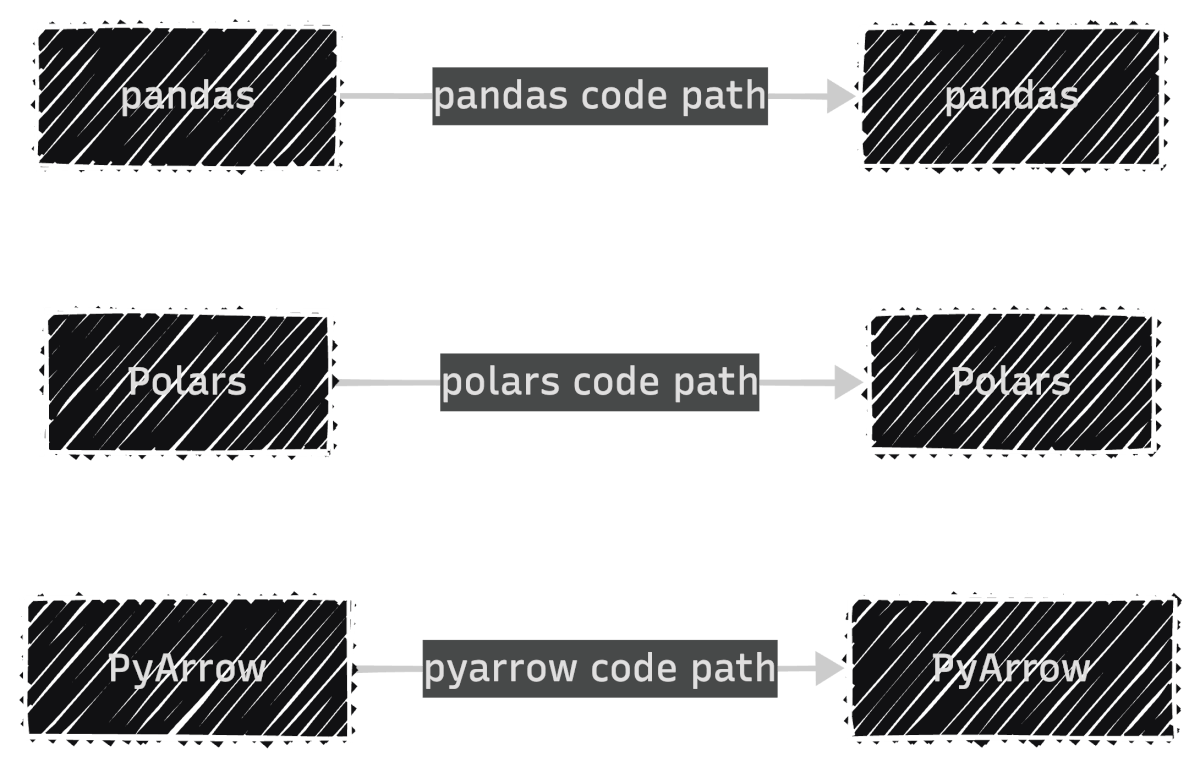
If you’re building a library, you don’t control which dataframe library your users prefer. Without Narwhals, you’d maintain separate implementations for each library:
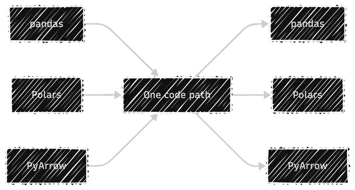
With Narwhals, one code path replaces all three, so every bug fix and feature update applies to all dataframe types at once:
To install Narwhals, run:
pip install narwhals
This article uses narwhals v2.16.0.
For more Narwhals examples across pandas, Polars, and PySpark, see Narwhals: Unified DataFrame Functions for pandas, Polars, and PySpark.
The from_native / to_native Pattern
The core pattern has three steps: convert the incoming dataframe to Narwhals, do your work, and convert back.
First, load a pandas DataFrame and wrap it with nw.from_native(). This gives you a Narwhals DataFrame with a Polars-like API:
import narwhals as nw
import pandas as pd

df_pd = pd.read_parquet("yellow_tripdata_2024-01.parquet")
df = nw.from_native(df_pd)
Next, use Narwhals’ API to define the analysis. The syntax mirrors Polars with nw.col(), .agg(), and .sort():
result = (
    df.group_by("payment_type")
    .agg(
        nw.col("fare_amount").sum().alias("total_fare"),
        nw.col("fare_amount").mean().alias("avg_fare"),
        nw.col("fare_amount").count().alias("trip_count"),
    )
    .sort("trip_count", descending=True)
)
Finally, call .to_native() to convert back to the original library. Since we started with pandas, we get a pandas DataFrame back:
print(result.to_native())
payment_type   total_fare   avg_fare  trip_count
1             1  43035538.92  18.557432     2319046
0             2   7846602.79  17.866037      439191
4             0   2805509.77  20.016194      140162
2             4     62243.19   1.334889       46628
3             3    132330.09   6.752569       19597
To see the real benefit, wrap this logic in a reusable function. It accepts any supported dataframe type, and Narwhals handles the rest:
def fare_summary(df_native):
    df = nw.from_native(df_native)
    return (
        df.group_by("payment_type")
        .agg(
            nw.col("fare_amount").sum().alias("total_fare"),
            nw.col("fare_amount").mean().alias("avg_fare"),
            nw.col("fare_amount").count().alias("trip_count"),
        )
        .sort("trip_count", descending=True)
        .to_native()
    )
Now the same function works with pandas, Polars, and PyArrow:
print(fare_summary(df_pd))
   payment_type    total_fare    avg_fare  trip_count
0             1  3.704733e+07   16.689498     2219230
1             2  7.352498e+06   15.411498      477083
2             0  1.396918e+06   19.569349       71382
3             4  1.280650e+05   15.671294        8173
4             3  1.108880e+04   12.906526         859
import polars as pl

df_pl = pl.read_parquet("yellow_tripdata_2024-01.parquet")
print(fare_summary(df_pl))
shape: (5, 4)
┌──────────────┬────────────┬───────────┬────────────┐
│ payment_type ┆ total_fare ┆ avg_fare  ┆ trip_count │
│ ---          ┆ ---        ┆ ---       ┆ ---        │
│ i64          ┆ f64        ┆ f64       ┆ u32        │
╞══════════════╪════════════╪═══════════╪════════════╡
│ 1            ┆ 4.3036e7   ┆ 18.557432 ┆ 2319046    │
│ 2            ┆ 7.8466e6   ┆ 17.866037 ┆ 439191     │
│ 0            ┆ 2.8055e6   ┆ 20.016194 ┆ 140162     │
│ 4            ┆ 62243.19   ┆ 1.334889  ┆ 46628      │
│ 3            ┆ 132330.09  ┆ 6.752569  ┆ 19597      │
└──────────────┴────────────┴───────────┴────────────┘
import duckdb

df_duck = duckdb.sql("SELECT * FROM 'yellow_tripdata_2024-01.parquet'")
print(fare_summary(df_duck))
┌──────────────┬────────────────────┬────────────────────┬────────────┐
│ payment_type │     total_fare     │      avg_fare      │ trip_count │
│    int64     │       double       │       double       │   int64    │
├──────────────┼────────────────────┼────────────────────┼────────────┤
│            1 │  43035538.92000025 │ 18.557432202724847 │    2319046 │
│            2 │    7846602.7900001 │  17.86603730495411 │     439191 │
│            0 │ 2805509.7700004894 │ 20.016193904200065 │     140162 │
│            4 │  62243.19000000006 │ 1.3348886934888922 │      46628 │
│            3 │ 132330.08999999985 │  6.752568760524563 │      19597 │
└──────────────┴────────────────────┴────────────────────┴────────────┘
Notice that the output type always matches the input. This is what makes Narwhals practical for library authors: users keep working with their preferred dataframe library, and your code stays the same.
For a detailed comparison of pandas, Polars, and DuckDB themselves, see pandas vs Polars vs DuckDB: A Data Scientist’s Guide.
The @narwhalify Decorator
For simpler cases, the @nw.narwhalify decorator handles the from_native/to_native boilerplate:
@nw.narwhalify
def high_fare_filter(df, threshold: float = 20.0):
    return (
        df.filter(nw.col("fare_amount") > threshold)
        .select("payment_type", "fare_amount", "trip_distance", "tip_amount")
        .sort("fare_amount", descending=True)
        .head(5)
    )

print(high_fare_filter(df_pd, threshold=50.0))
   payment_type  fare_amount  trip_distance  tip_amount
0             2     401200.0          42.39        0.00
1             1        398.0          39.49       50.00
2             1        397.5          42.83       50.00
3             1        384.5          45.33       77.60
4             1        363.0          32.43       73.30
Real-World Adoption
Narwhals has seen wide adoption across the Python ecosystem. Over 25 libraries use it, including:
- Visualization: Altair, Plotly, Bokeh
- ML: scikit-lego, fairlearn
- Interactive: marimo
- Forecasting: darts, hierarchicalforecast
These libraries accept any dataframe type from users because Narwhals handles the compatibility layer with zero additional dependencies.
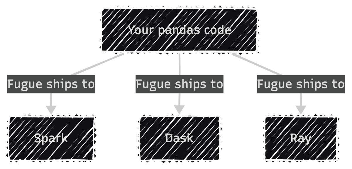
Fugue: Keep Your Code, Swap the Engine
Fugue focuses on scaling existing code to distributed engines:
- What it does: Ships your pandas functions to Spark, Dask, or Ray without rewriting them
- How it works: Uses type annotations to infer input/output schemas, then translates execution to the target engine
- Who it’s for: Data engineers who already have pandas pipelines and need to scale them
In other words, your existing pandas code runs as-is on distributed engines:
To install Fugue, run:
pip install fugue
This article uses fugue v0.9.6.
The transform() Pattern
With Fugue, you begin with a regular pandas function. No Fugue imports or special decorators needed. The only requirement is type annotations, which tell Fugue how to handle the data when it runs on a different engine:
import pandas as pd


def fare_summary(df: pd.DataFrame) -> pd.DataFrame:
    return (
        df.groupby("payment_type")
        .agg(
            total_fare=("fare_amount", "sum"),
            avg_fare=("fare_amount", "mean"),
            trip_count=("fare_amount", "count"),
        )
        .reset_index()
        .sort_values("trip_count", ascending=False)
    )
Since this is plain pandas, you can test it locally as you normally would:
input_df = pd.read_parquet("yellow_tripdata_2024-01.parquet")
result = fare_summary(input_df)
print(result)
   payment_type   total_fare   avg_fare  trip_count
1             1  43035538.92  18.557432     2319046
2             2   7846602.79  17.866037      439191
0             0   2805509.77  20.016194      140162
4             4     62243.19   1.334889       46628
3             3    132330.09   6.752569       19597
To scale this to Spark, pass the function through Fugue’s transform() with a different engine:
from fugue import transform

# Scale to Spark: same function, different engine
result_spark = transform(
    input_df,
    fare_summary,
    schema="payment_type:int,total_fare:double,avg_fare:double,trip_count:long",
    engine="spark",
)

result_spark.show()
+------------+----------+--------+----------+
|payment_type|total_fare|avg_fare|trip_count|
+------------+----------+--------+----------+
|           1| 43035539 |  18.56 |   2319046|
|           2|  7846603 |  17.87 |    439191|
|           0|  2805510 |  20.02 |    140162|
|           4|    62243 |   1.33 |     46628|
|           3|   132330 |   6.75 |     19597|
+------------+----------+--------+----------+
The schema parameter is required for distributed engines because frameworks like Spark need to know column types before execution. This is a constraint of distributed computing, not Fugue itself.
Scaling to DuckDB
For local speedups without distributed infrastructure, Fugue also supports DuckDB as an engine:
result_duck = transform(
    input_df,
    fare_summary,
    schema="payment_type:int,total_fare:double,avg_fare:double,trip_count:long",
    engine="duckdb",
)
print(result_duck)
   payment_type   total_fare   avg_fare  trip_count
0             1  43035538.92  18.557432     2319046
1             2   7846602.79  17.866037      439191
2             0   2805509.77  20.016194      140162
3             4     62243.19   1.334889       46628
4             3    132330.09   6.752569       19597
Notice that the function never changes. Fugue handles the conversion between pandas and each engine automatically.
FugueSQL
Fugue also includes FugueSQL, which lets you write SQL that calls Python functions. To use it, install Fugue with the SQL extra:
pip install 'fugue[sql]'
This article uses fugue v0.9.6.
This is useful for teams that prefer SQL but need custom transformations:
from fugue.api import fugue_sql

result = fugue_sql("""
    SELECT payment_type, fare_amount, trip_distance
    FROM input_df
    WHERE fare_amount > 50
    ORDER BY fare_amount DESC
    LIMIT 5
""")
print(result)
         payment_type  fare_amount  trip_distance
1714869             3       5000.0            0.0
1714870             3       5000.0            0.0
1714871             3       2500.0            0.0
1714873             1       2500.0            0.0
2084560             1       2500.0            0.0
Summary
| Tool | Choose when you need to… | Strengths |
|---|---|---|
| Ibis | Query SQL databases, deploy from local to cloud, or want one API across 22+ backends | Compiles to native SQL; DuckDB locally, BigQuery/Snowflake in production |
| Narwhals | Build a library that accepts any dataframe type | Zero dependencies, negligible overhead, battle-tested in 25+ libraries |
| Fugue | Scale existing pandas code to Spark, Dask, or Ray, or mix SQL with Python | Keep your functions unchanged, just swap the engine |
The key distinction is the type of backend each tool targets: SQL databases (Ibis), dataframe libraries (Narwhals), or distributed engines (Fugue). Once you know which backend type you need, the choice becomes straightforward.
Related Tutorials
- Cloud Scaling: Coiled: Scale Python Data Pipeline to the Cloud in Minutes for deploying Dask workloads to the cloud
📚 Want to go deeper? My book shows you how to build data science projects that actually make it to production. Get the book →
Stay Current with CodeCut
Actionable Python tips, curated for busy data pros. Skim in under 2 minutes, three times a week.