Generic selectors
Exact matches only
Search in title
Search in content
Post Type Selectors
Filter by Categories
About Article
Analyze Data
Archive
Best Practices
Better Outputs
Blog
Code Optimization
Code Quality
Command Line
Daily tips
Dashboard
Data Analysis & Manipulation
Data Engineer
Data Visualization
DataFrame
Delta Lake
DevOps
DuckDB
Environment Management
Feature Engineer
Git
Jupyter Notebook
LLM
LLM
Machine Learning
Machine Learning
Machine Learning & AI
Manage Data
MLOps
Natural Language Processing
NumPy
Pandas
Polars
PySpark
Python Tips
Python Utilities
Python Utilities
Scrape Data
SQL
Testing
Time Series
Tools
Visualization
Visualization & Reporting
Workflow & Automation
Workflow Automation

Machine Learning

Hydra: YAML-Based Config Management Made Simple

Want to experiment with different data processing methods and model hyperparameters? Manually editing the configuration file each time can be a hassle.

Hydra lets you compose configurations quickly and easily by selecting options from different config groups. You can have groups for processing, model hyperparameters, and databases, each with multiple options like process1.yaml and process2.yaml.

Hydra: YAML-Based Config Management Made Simple Read More »

TimberTrek: Create an Interactive and Comprehensive Decision Tree

Complex decision tree ensembles like random forests and gradient-boosted trees can be hard to understand and interpret. This results in difficulties for data scientists in making informed decisions about model refinement or deployment.

TimberTrek helps address this issue by providing an interactive visualization tool for exploring and comparing multiple decision tree models.

It also lets users filter and select models based on custom criteria (e.g., fairness, simplicity).

Link to TimberTrek.
Favorite

TimberTrek: Create an Interactive and Comprehensive Decision Tree Read More »

Rapid Prototyping and Comparison of Basic Models with Lazy Predict

Traditionally, data scientists need to manually code and test multiple models, which is time-consuming and labor-intensive.

Lazy Predict enables rapid prototyping and comparison of multiple basic models without extensive manual coding or parameter tuning.

This helps data scientists identify promising approaches and iterate on them more quickly.

Here’s a practical example using the breast cancer dataset:

from lazypredict.Supervised import LazyClassifier
from sklearn.datasets import load_breast_cancer
from sklearn.model_selection import train_test_split

data = load_breast_cancer()
X = data.data
y= data.target

X_train, X_test, y_train, y_test = train_test_split(X, y,test_size=.5,random_state =123)

clf = LazyClassifier(verbose=0, ignore_warnings=True, custom_metric=None)
models, predictions = clf.fit(X_train, X_test, y_train, y_test)

print(models)

This code snippet generates a comprehensive comparison of various classification models, evaluating them on metrics such as accuracy, balanced accuracy, ROC AUC, and F1 score. The output is a table ranking models by performance, allowing quick identification of the most promising algorithms for the given dataset.

| Model | Accuracy | Balanced Accuracy | ROC AUC | F1 Score | Time Taken |
|:——————————-|———–:|——————–:|———-:|———–:|————-:|
| LinearSVC | 0.989474 | 0.987544 | 0.987544 | 0.989462 | 0.0150008 |
| SGDClassifier | 0.989474 | 0.987544 | 0.987544 | 0.989462 | 0.0109992 |
| MLPClassifier | 0.985965 | 0.986904 | 0.986904 | 0.985994 | 0.426 |
| Perceptron | 0.985965 | 0.984797 | 0.984797 | 0.985965 | 0.0120046 |
| LogisticRegression | 0.985965 | 0.98269 | 0.98269 | 0.985934 | 0.0200036 |
| LogisticRegressionCV | 0.985965 | 0.98269 | 0.98269 | 0.985934 | 0.262997 |
| SVC | 0.982456 | 0.979942 | 0.979942 | 0.982437 | 0.0140011 |
| CalibratedClassifierCV | 0.982456 | 0.975728 | 0.975728 | 0.982357 | 0.0350015 |
| PassiveAggressiveClassifier | 0.975439 | 0.974448 | 0.974448 | 0.975464 | 0.0130005 |
| LabelPropagation | 0.975439 | 0.974448 | 0.974448 | 0.975464 | 0.0429988 |
| LabelSpreading | 0.975439 | 0.974448 | 0.974448 | 0.975464 | 0.0310006 |
| RandomForestClassifier | 0.97193 | 0.969594 | 0.969594 | 0.97193 | 0.033 |
| GradientBoostingClassifier | 0.97193 | 0.967486 | 0.967486 | 0.971869 | 0.166998 |
| QuadraticDiscriminantAnalysis | 0.964912 | 0.966206 | 0.966206 | 0.965052 | 0.0119994 |
| HistGradientBoostingClassifier | 0.968421 | 0.964739 | 0.964739 | 0.968387 | 0.682003 |
| RidgeClassifierCV | 0.97193 | 0.963272 | 0.963272 | 0.971736 | 0.0130029 |
| RidgeClassifier | 0.968421 | 0.960525 | 0.960525 | 0.968242 | 0.0119977 |
| AdaBoostClassifier | 0.961404 | 0.959245 | 0.959245 | 0.961444 | 0.204998 |
| ExtraTreesClassifier | 0.961404 | 0.957138 | 0.957138 | 0.961362 | 0.0270066 |
| KNeighborsClassifier | 0.961404 | 0.95503 | 0.95503 | 0.961276 | 0.0560005 |
| BaggingClassifier | 0.947368 | 0.954577 | 0.954577 | 0.947882 | 0.0559971 |
| BernoulliNB | 0.950877 | 0.951003 | 0.951003 | 0.951072 | 0.0169988 |
| LinearDiscriminantAnalysis | 0.961404 | 0.950816 | 0.950816 | 0.961089 | 0.0199995 |
| GaussianNB | 0.954386 | 0.949536 | 0.949536 | 0.954337 | 0.0139935 |
| NuSVC | 0.954386 | 0.943215 | 0.943215 | 0.954014 | 0.019989 |
| DecisionTreeClassifier | 0.936842 | 0.933693 | 0.933693 | 0.936971 | 0.0170023 |
| NearestCentroid | 0.947368 | 0.933506 | 0.933506 | 0.946801 | 0.0160074 |
| ExtraTreeClassifier | 0.922807 | 0.912168 | 0.912168 | 0.922462 | 0.0109999 |
| CheckingClassifier | 0.361404 | 0.5 | 0.5 | 0.191879 | 0.0170043 |
| DummyClassifier | 0.512281 | 0.489598 | 0.489598 | 0.518924 | 0.0119965 |

The top-performing models in this case are:

LinearSVC (Accuracy: 0.989, ROC AUC: 0.988)

SGDClassifier (Accuracy: 0.989, ROC AUC: 0.988)

MLPClassifier (Accuracy: 0.986, ROC AUC: 0.987)

Link to Lazy Predict.
Favorite

Rapid Prototyping and Comparison of Basic Models with Lazy Predict Read More »

modelstore: A Unified Solution for Cloud and Local Model Storage

Different cloud providers and storage systems require unique implementation methods, making retrieving and loading stored models for deployment or further use complex. 

modelstore offers a unified interface for storing models across multiple cloud platforms (AWS, GCP, Azure) and local storage. It provides easy methods to download models by ID or load them directly into memory.

modelstore supports the following storages:

AWS S3 Bucket

Azure Blob Storage

Google Cloud Storage Bucket

Any s3-compatible object storage that you can access via MinIO

A filesystem directory

Here is an example of how to use modelstore:

from modelstore import ModelStore

# Train your model
clf = RandomForestClassifier(n_estimators=10)
clf.fit(X, Y)

# Create a model store with a GCP bucket
model_store = ModelStore.from_gcloud(
project_name="my-project",
bucket_name="my-bucket",
)

# Upload the model to your model store
domain = "example-model"
meta_data = model_store.upload(domain, model=clf)

# Load the model back
clf = model_store.load(
domain=model_domain,
model_id=meta["model"]["model_id"]
)

Link to modelstore.
Favorite

modelstore: A Unified Solution for Cloud and Local Model Storage Read More »

Simplifying ML Model Integration with FastAPI

Motivation

Imagine this scenario: You have just built an ML model with great performance, and you want to share this model with your team members so that they can develop a web application on top of your model.

One way to share the model with your team members is to save the model to a file (e.g., using pickle, joblib, or framework-specific methods) and share the file directly

import joblib

model = …

# Save model
joblib.dump(model, "model.joblib")

# Load model
model = joblib.load(model)

However, this approach requires the same environment and dependencies, and it can pose potential security risks.

An alternative is creating an API for your ML model. APIs define how software components interact, allowing:

Access from various programming languages and platforms

Easier integration for developers unfamiliar with ML or Python

Versatile use across different applications (web, mobile, etc.)

This approach simplifies model sharing and usage, making it more accessible for diverse development needs.

Create an ML API with FastAPI

Let’s learn how to create an ML API with FastAPI, a modern and fast web framework for building APIs with Python.

Before we begin constructing an API for a machine learning model, let’s first develop a basic model that our API will use. In this example, we’ll create a model that predicts the median house price in California.

from sklearn.datasets import fetch_california_housing
from sklearn.model_selection import train_test_split
from sklearn.linear_model import LinearRegression
from sklearn.metrics import mean_squared_error
import joblib

# Load dataset
X, y = fetch_california_housing(as_frame=True, return_X_y=True)

# Split dataset into training and test sets
X_train, X_test, y_train, y_test = train_test_split(
X, y, test_size=0.2, random_state=42
)

# Initialize and train the logistic regression model
model = LinearRegression()
model.fit(X_train, y_train)

# Predict and evaluate the model
y_pred = model.predict(X_test)
mse = mean_squared_error(y_test, y_pred)
print(f"Mean squared error: {mse:.2f}")

# Save model
joblib.dump(model, "lr.joblib")

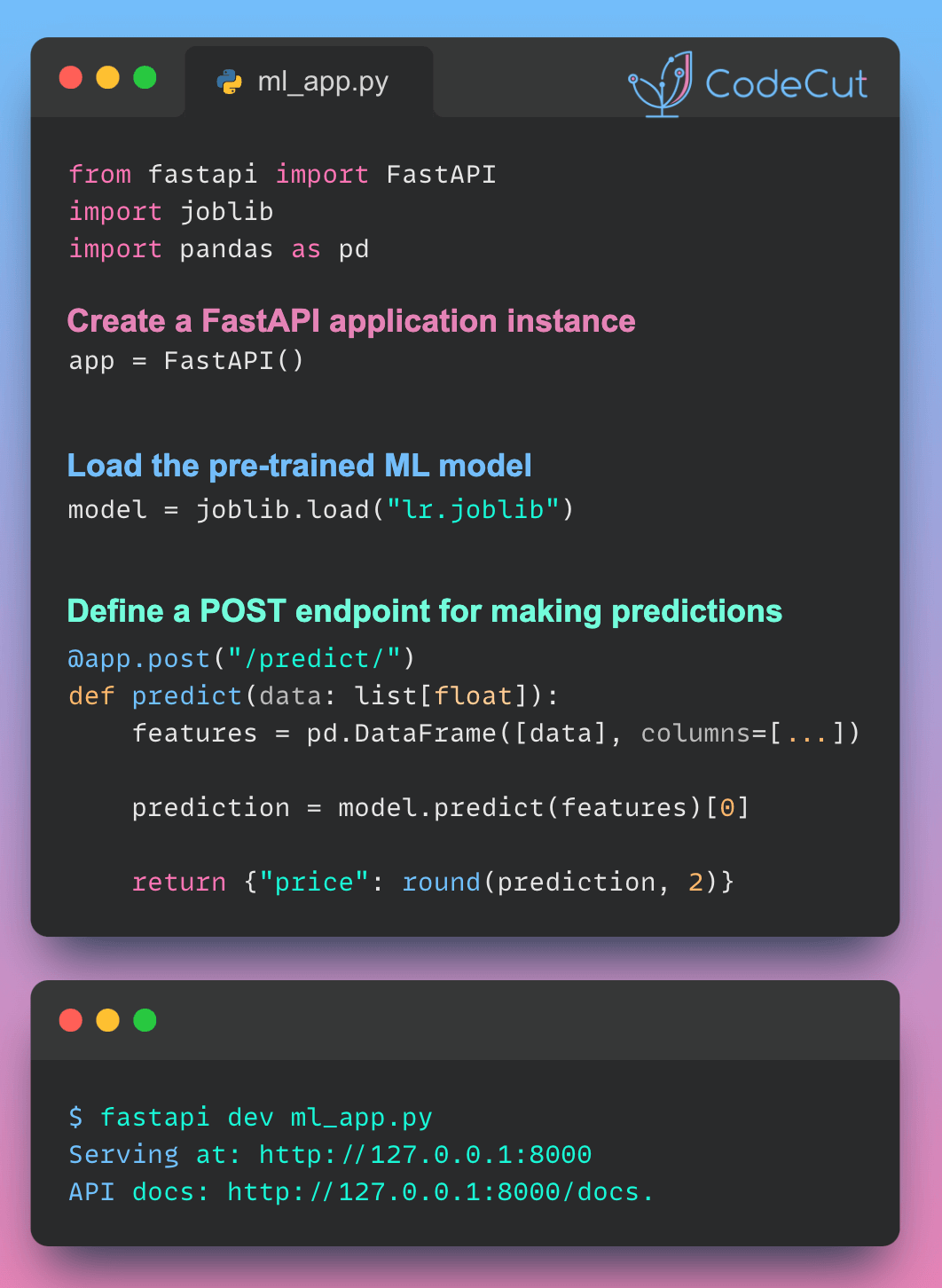
Once we have our model, we can create an API for it using FastAPI. We’ll define a POST endpoint for making predictions and use the model to make predictions.

Here’s an example of how to create an API for a machine learning model using FastAPI:

%%writefile ml_app.py
from fastapi import FastAPI
import joblib
import pandas as pd

# Create a FastAPI application instance
app = FastAPI()

# Load the pre-trained machine learning model
model = joblib.load("lr.joblib")

# Define a POST endpoint for making predictions
@app.post("/predict/")
def predict(data: list[float]):
# Define the column names for the input features
columns = [
"MedInc",
"HouseAge",
"AveRooms",
"AveBedrms",
"Population",
"AveOccup",
"Latitude",
"Longitude",
]

# Create a pandas DataFrame from the input data
features = pd.DataFrame([data], columns=columns)

# Use the model to make a prediction
prediction = model.predict(features)[0]

# Return the prediction as a JSON object, rounding to 2 decimal places
return {"price": round(prediction, 2)}

To run your FastAPI app for development, use the fastapi dev command:

$ fastapi dev ml_app.py

This will start the development server and open the API documentation in your default browser.

You can now use the API to make predictions by sending a POST request to the /predict/ endpoint with the input data. For example:

Running this cURL command on your terminal:

curl -X 'POST' \
'http://127.0.0.1:8000/predict/' \
-H 'accept: application/json' \
-H 'Content-Type: application/json' \
-d '[
1.68, 25, 4, 2, 1400, 3, 36.06, -119.01
]'

This will return the predicted price as a JSON object, rounded to 2 decimal places:

{"price":1.51}
Favorite

Simplifying ML Model Integration with FastAPI Read More »

Model Logging Made Easy: MLflow vs. Pickle

Using MLflow to log models offers distinct advantages over Pickle. Here’s a detailed look at the benefits:

Managing Library Versions

Problem

Different machine learning models may depend on various versions of the same library, leading to compatibility conflicts. Manually tracking and configuring the correct environment for each model can be tedious and error-prone.

Solution

MLflow automatically logs all dependencies, allowing users to easily recreate the exact environment necessary to run the model. This feature simplifies deployment and enhances reproducibility.

Documenting Inputs and Outputs

Problem

The expected inputs and outputs of a model are often not well-documented, making it challenging for others to utilize the model correctly.

Solution

MLflow defines a clear schema for inputs and outputs, ensuring that users know precisely what data to provide and what to expect in return. This clarity fosters better collaboration and reduces confusion.

Example Implementation

To demonstrate the advantages of MLflow, let’s implement a simple logistic regression model and log it.

Logging the Model

import mlflow
from mlflow.models import infer_signature
import numpy as np
from sklearn.linear_model import LogisticRegression

with mlflow.start_run():
   X = np.array([-2, -1, 0, 1, 2, 1]).reshape(-1, 1)
   y = np.array([0, 0, 1, 1, 1, 0])
   lr = LogisticRegression()
   lr.fit(X, y)
   signature = infer_signature(X, lr.predict(X))

   model_info = mlflow.sklearn.log_model(
       sk_model=lr, artifact_path="model", signature=signature
  )

   print(f"Saving data to {model_info.model_uri}")

This code will output the location where the model is saved:

Saving data to runs:/f8b0fc900aa14cf0ade8d0165c5a9f11/model

Using the Logged Model

To use the logged model later, you can load it with the model_uri:

import mlflow
import numpy as np

model_uri = "runs:/1e20d72afccf450faa3b8a9806a97e83/model"
sklearn_pyfunc = mlflow.pyfunc.load_model(model_uri=model_uri)

data = np.array([-4, 1, 0, 10, -2, 1]).reshape(-1, 1)
predictions = sklearn_pyfunc.predict(data)

Inspecting Model Artifacts

Check the saved artifacts in mlruns/0/1e20d72afccf450faa3b8a9806a97e83/artifacts/model:

MLmodel model.pkl requirements.txt
conda.yaml python_env.yaml

Understanding Model Configuration

The MLmodel file contains critical information about the model, including its dependencies and input/output specifications:

artifact_path: model
flavors:
python_function:
env:
conda: conda.yaml
virtualenv: python_env.yaml
loader_module: mlflow.sklearn
model_path: model.pkl
predict_fn: predict
python_version: 3.11.6
sklearn:
code: null
pickled_model: model.pkl
serialization_format: cloudpickle
sklearn_version: 1.4.1.post1
mlflow_version: 2.15.0
model_size_bytes: 722
model_uuid: e7487bc3c4ab417c965144efcecaca2f
run_id: 1e20d72afccf450faa3b8a9806a97e83
signature:
inputs: '[{"type": "tensor", "tensor-spec": {"dtype": "int64", "shape": [-1, 1]}}]'
outputs: '[{"type": "tensor", "tensor-spec": {"dtype": "int64", "shape": [-1]}}]'
params: null
utc_time_created: '2024-08-02 20:58:16.516963'

Environment Specifications

The conda.yaml and python_env.yaml files detail the dependencies required for the model, ensuring a consistent runtime environment. Here’s a look at conda.yaml:

# conda.yaml
channels:
– conda-forge
dependencies:
– python=3.11.6
– pip<=24.2
– pip:
– mlflow==2.15.0
– cloudpickle==2.2.1
– numpy==1.23.5
– psutil==5.9.6
– scikit-learn==1.4.1.post1
– scipy==1.11.3
name: mlflow-env

And for python_env.yaml and requirements.txt:

# python_env.yaml
python: 3.11.6
build_dependencies:
– pip==24.2
– setuptools
– wheel==0.40.0
dependencies:
– -r requirements.txt

# requirements.txt
mlflow==2.15.0
cloudpickle==2.2.1
numpy==1.23.5
psutil==5.9.6
scikit-learn==1.4.1.post1
scipy==1.11.3

Learn more about MLFlow Models.

Favorite

Model Logging Made Easy: MLflow vs. Pickle Read More »

UMAP: Transforming Multi-Dimensional Data into Comprehensive 2D Plots

Visualizing multi-dimensional datasets can be challenging. UMAP provides a solution by reducing the dimensions of your dataset to create 2D representations.

The scatter plot displayed above represents the fruit dataset, which originally contains four distinct features. By compressing it from four dimensions down to two, we can easily see four clusters that represent each type of fruit.

Link to UMAP.
Favorite

UMAP: Transforming Multi-Dimensional Data into Comprehensive 2D Plots Read More »

MLflow Model Registry: A Centralized Platform for Managing Machine Learning Models

MLflow Model Registry is an extension of MLflow Tracking that allows you to store and categorize machine learning models using version control, aliases, and tags.

Once a model has been selected, it can be easily deployed as a service on the host, making it accessible for use in production environments.

Learn more about MLflow model registry.
Favorite

MLflow Model Registry: A Centralized Platform for Managing Machine Learning Models Read More »

KitOps: A Unified Solution to Manage AI/ML Projects

In AI/ML projects, various components are usually stored in separate locations:

Code resides in Git repositories

Datasets and models are stored in DVC or storage services like S3

Parameters are managed using experiment management tools

As components are stored separately, the process of deploying and integrating them can become more complicated.

KitOps’s ModelKits offers a unified solution by packaging these components into ModelKits. This allows for easy versioning and sharing of components with other team members in just a few commands.

Learn more about KitOps.
Favorite

KitOps: A Unified Solution to Manage AI/ML Projects Read More »

0
    0
    Your Cart
    Your cart is empty
    Scroll to Top

    Work with Khuyen Tran

    Work with Khuyen Tran