Time Series Archives

Extract Dates from Text with Datefinder

2 Comments / Natural Language Processing / Khuyen Tran

Motivation

Extracting dates from unstructured text can be a frustrating and error-prone task when dates appear in varying formats. For example:

# Example Input
string_with_dates = """
We have one meeting on May 17th, 2021 at 9:00am
and another meeting on 5/18/2021 at 10:00.
I hope you can attend one of the meetings.
"""

# Traditional string processing to find dates
import re

# Basic regex for dates
pattern = r"(\b\d{1,2}/\d{1,2}/\d{4}\b)|(\b\w+\s\d{1,2}(st|nd|rd|th)?,\s\d{4}\b)"
matches = re.findall(pattern, string_with_dates)
print(f"Matches: {[match[0] or match[1] for match in matches]}") # Limited and inflexible

Output:

Matches: ['May 17th, 2021', '5/18/2021']

Using basic regular expressions, the extracted dates are limited and often incomplete, especially when handling a variety of date formats. This makes it difficult to consistently extract and process dates from large, diverse datasets.

Introduction to Datefinder

Datefinder is a Python library designed to simplify the extraction of dates from text. It intelligently detects date-like strings and converts them into Python datetime objects, handling a wide range of formats automatically.

To install Datefinder, simply use the following command:

pip install datefinder

In this post, we will explore how Datefinder can be used to efficiently extract dates from unstructured text.

Extracting Dates from Text

Datefinder makes the process of identifying and extracting dates straightforward, even when the formats vary within the text. Below is an example demonstrating its use.

import datefinder

# Example Input
string_with_dates = """
We have one meeting on May 17th, 2021 at 9:00am
and another meeting on 5/18/2021 at 10:00.
I hope you can attend one of the meetings.
"""

# Extract dates from text
matches = datefinder.find_dates(string_with_dates)

# Print each match
for match in matches:
print(match)

In the above code:

datefinder.find_dates() scans the input text for potential date strings.

The string_with_dates variable contains examples of multiple date formats.

The matches iterator yields each identified date as a Python datetime object.

When you run the above code, Datefinder will identify and extract both dates:

2021-05-17 09:00:00
2021-05-18 10:00:00

Datefinder not only detects the dates but also converts them into a standard, machine-readable format (datetime objects), which can then be used for further processing or analysis.

Conclusion

Datefinder is a powerful tool for extracting dates from unstructured text. It simplifies the process by handling various date formats and converting them into datetime objects. Whether you’re working on NLP tasks, data preprocessing, or automating workflows that involve date extraction, Datefinder saves time and effort.

Link to Datefinder.
Favorite

Extract Dates from Text with Datefinder Read More »

MLForecast: Automate External Feature Handling

3 Comments / Time Series / Khuyen Tran

Motivation

Time series forecasting often requires incorporating external factors that can influence the target variable. However, handling these external factors (exogenous features) can be complex, especially when some features remain constant while others change over time.

# Example without proper handling of exogenous features
import pandas as pd

# Sales data with product info and prices
data = pd.DataFrame({
'date': ['2024-01-01', '2024-01-02', '2024-01-03'],
'product_id': [1, 1, 1],
'category': ['electronics', 'electronics', 'electronics'],
'price': [99.99, 89.99, 94.99],
'sales': [150, 200, 175]
})

# Difficult to handle static (category) vs dynamic (price) features
# Risk of data leakage or incorrect feature engineering

This code shows the challenge of handling both static features (product category) and dynamic features (price) in time series forecasting. Without proper handling, you might incorrectly use future information or miss important patterns in the data.

Understanding Features in Time Series

Before diving into MLForecast, let’s understand two important concepts:

Static features: These are features that don’t change over time (like product category or location)

Dynamic features (exogenous): These are features that change over time (like price or weather)

Introduction to MLForecast

MLForecast is a Python library that simplifies time series forecasting with machine learning models while properly handling both static and dynamic features. It can be installed using:

pip install mlforecast

As covered in the past article about MLForecast’s workflow, it provides an integrated approach to time series forecasting. In this post, we will focus on its exogenous features capabilities.

Working with Exogenous Features

MLForecast makes it easy to handle both static and dynamic features in your forecasting models. Here’s how:

First, let’s prepare our data with both types of features:

import lightgbm as lgb
from mlforecast import MLForecast
from mlforecast.utils import generate_daily_series, generate_prices_for_series

# Generate sample data
series = generate_daily_series(100, equal_ends=True, n_static_features=2)
series = series.rename(columns={"static_0": "store_id", "static_1": "product_id"})

# Generate price catalog (dynamic feature)
prices_catalog = generate_prices_for_series(series)

# Merge static and dynamic features
series_with_prices = series.merge(prices_catalog, how='left')
print(series_with_prices.head(10))

Output:

unique_id ds y store_id product_id price
0 id_00 2000-10-05 39.811983 79 45 0.548814
1 id_00 2000-10-06 103.274013 79 45 0.715189
2 id_00 2000-10-07 176.574744 79 45 0.602763
3 id_00 2000-10-08 258.987900 79 45 0.544883
4 id_00 2000-10-09 344.940404 79 45 0.423655
5 id_00 2000-10-10 413.520305 79 45 0.645894
6 id_00 2000-10-11 506.990093 79 45 0.437587
7 id_00 2000-10-12 12.688070 79 45 0.891773
8 id_00 2000-10-13 111.133819 79 45 0.963663
9 id_00 2000-10-14 197.982842 79 45 0.383442

Now, let’s create and train our model:

# Create MLForecast model
fcst = MLForecast(
models=lgb.LGBMRegressor(random_state=0),
freq="D",
lags=[7], # Use 7-day lag
date_features=["dayofweek"], # Add day of week as feature
)

# Fit model specifying which features are static
fcst.fit(
series_with_prices,
static_features=["store_id", "product_id"], # Specify static features
)

# Check which features are used for training
print("\nFeatures used for training:")
print(fcst.ts.features_order_)

Output:

Features used for training:
['store_id', 'product_id', 'price', 'lag7', 'dayofweek']

Generate predictions:

# Make predictions using future prices
predictions = fcst.predict(
h=7, # Forecast 7 days ahead
X_df=prices_catalog # Provide future prices
)
predictions.head(10)

Output:

unique_id ds LGBMRegressor
0 id_00 2001-05-15 421.301684
1 id_00 2001-05-16 497.335181
2 id_00 2001-05-17 20.108545
3 id_00 2001-05-18 101.930145
4 id_00 2001-05-19 184.264253
5 id_00 2001-05-20 260.803990
6 id_00 2001-05-21 343.501305
7 id_01 2001-05-15 118.299009
8 id_01 2001-05-16 148.793503
9 id_01 2001-05-17 184.066779

The output shows forecasted values that take into account both static features (product information) and dynamic features (prices).

MLForecast vs Traditional Approaches

Traditional approaches often require separate handling of static and dynamic features, leading to complex preprocessing pipelines. MLForecast simplifies this by:

Automatically managing feature types

Preventing data leakage

Providing an integrated workflow

Conclusion

MLForecast’s handling of exogenous features significantly simplifies time series forecasting by providing a clean interface for both static and dynamic features. This makes it easier to incorporate external information into your forecasts while maintaining proper time series practices.

Link to MLForecast
Favorite

MLForecast: Automate External Feature Handling Read More »

Enhancing Predictive Models with Workalendar’s Holiday Handling

Leave a Comment / Time Series / Khuyen Tran

Incorporating holiday and working day information into predictive models can enhance accuracy, but it’s challenging due to regional variations in holiday schedules.

Workalendar simplifies this process by handling working days, holidays, and business calendars for various countries and regions.

Here are some examples:

Get US holidays in 2024:

from datetime import date
from workalendar.usa import UnitedStates

US_cal = UnitedStates()
US_cal.holidays(2024)

[(datetime.date(2024, 1, 1), 'New year'),
(datetime.date(2024, 1, 15), 'Birthday of Martin Luther King, Jr.'),
(datetime.date(2024, 2, 19), "Washington's Birthday"),
(datetime.date(2024, 5, 27), 'Memorial Day'),
(datetime.date(2024, 7, 4), 'Independence Day'),
(datetime.date(2024, 9, 2), 'Labor Day'),
(datetime.date(2024, 10, 14), 'Columbus Day'),
(datetime.date(2024, 11, 11), 'Veterans Day'),
(datetime.date(2024, 11, 28), 'Thanksgiving Day'),
(datetime.date(2024, 12, 25), 'Christmas Day')]

Check if a date is a working day:

US_cal.is_working_day(date(2024, 9, 15)) # Sunday

False

US_cal.is_working_day(date(2024, 9, 2)) # Labor Day

False

Calculate the number of working days between two dates, excluding weekends and holidays:

# Calculate working days between 2024/1/19 and 2024/5/15
US_cal.get_working_days_delta(date(2024, 1, 19), date(2024, 5, 15))

Get Japan holidays in 2024:

from workalendar.asia import Japan

# Get holidays in Japan
JA_cal = Japan()
JA_cal.holidays(2024)

[(datetime.date(2024, 1, 1), 'New year'),
(datetime.date(2024, 1, 8), 'Coming of Age Day'),
(datetime.date(2024, 2, 11), 'Foundation Day'),
(datetime.date(2024, 2, 23), "The Emperor's Birthday"),
(datetime.date(2024, 3, 20), 'Vernal Equinox Day'),
(datetime.date(2024, 4, 29), 'Showa Day'),
(datetime.date(2024, 5, 3), 'Constitution Memorial Day'),
(datetime.date(2024, 5, 4), 'Greenery Day'),
(datetime.date(2024, 5, 5), "Children's Day"),
(datetime.date(2024, 7, 15), 'Marine Day'),
(datetime.date(2024, 8, 11), 'Mountain Day'),
(datetime.date(2024, 9, 16), 'Respect-for-the-Aged Day'),
(datetime.date(2024, 9, 22), 'Autumnal Equinox Day'),
(datetime.date(2024, 10, 14), 'Sports Day'),
(datetime.date(2024, 11, 3), 'Culture Day'),
(datetime.date(2024, 11, 23), 'Labour Thanksgiving Day')]

Link to Workalendar.

Next Step

If you liked this blog post, you might also like:

Pendulum: Python Datetimes Made Easy – For intuitive datetime handling and timezone management.

Maya: Convert the string to datetime automatically – For effortless string-to-datetime conversion.

Datefinder: Automatically Find Dates and Time in a Python String – For extracting dates from text.

Favorite

Enhancing Predictive Models with Workalendar’s Holiday Handling Read More »

Avoiding Data Leakage in Time Series Analysis with TimeSeriesSplit

Leave a Comment / Feature Engineer, Time Series / Khuyen Tran

Time series data is unique because it has a temporal order. This means that data from the future shouldn’t influence predictions about the past. However, standard cross-validation techniques like K-Fold randomly shuffle the data, potentially using future information to predict past events.

scikit-learn’s TimeSeriesSplit is a specialized cross-validator for time series data. It respects the temporal order of our data, ensuring that we always train on past data and test on future data.

Let’s explore how to use TimeSeriesSplit with a simple example:

import numpy as np
from sklearn.model_selection import TimeSeriesSplit

X = np.array([[1, 2], [3, 4], [1, 2], [3, 4], [1, 2], [3, 4]])
y = np.array([1, 2, 3, 4, 5, 6])

tscv = TimeSeriesSplit(n_splits=3)

for i, (train_index, test_index) in enumerate(tscv.split(X)):
print(f"Fold {i}:")
print(f" Train: index={train_index}")
print(f" Test: index={test_index}")

Fold 0:
Train: index=[0 1 2]
Test: index=[3]
Fold 1:
Train: index=[0 1 2 3]
Test: index=[4]
Fold 2:
Train: index=[0 1 2 3 4]
Test: index=[5]

From the outputs, we can see that:

Temporal Integrity: The split always respects the original order of the data.

Growing Training Set: With each fold, the training set expands to include more historical data.

Forward-Moving Test Set: The test set is always a single future sample, progressing with each fold.

No Data Leakage: Future information is never used to predict past events.

This approach mimics real-world forecasting scenarios, where models use historical data to predict future outcomes.
Favorite

Avoiding Data Leakage in Time Series Analysis with TimeSeriesSplit Read More »

Pendulum: Python Datetimes Made Easy

1 Comment / Time Series / Khuyen Tran

While Python’s built-in datetime library is sufficient for basic use cases, it can become cumbersome when dealing with more complex scenarios.

Pendulum offers a more intuitive and user-friendly API, serving as a convenient drop-in replacement for the standard datetime class.

Here’s a comparison of syntax and functionality between the standard datetime library and Pendulum:

Creating a datetime

Datetime:

from datetime import datetime
now = datetime.now()

Pendulum:

import pendulum
now = pendulum.now()

Date arithmetic

Datetime:

from datetime import timedelta
future = now + timedelta(days=7)

Pendulum:

future = now.add(days=7)

Timezone handling: Datetime (with pytz):

import pytz
utc_now = datetime.now(pytz.UTC)
tokyo_tz = pytz.timezone('Asia/Tokyo')
tokyo_time = utc_now.astimezone(tokyo_tz)

Pendulum:

tokyo_time = now.in_timezone("Asia/Tokyo")

Parsing dates

Datetime:

parsed = datetime.strptime("2023-05-15 14:30:00", "%Y-%m-%d %H:%M:%S")
parsed = pytz.UTC.localize(parsed)

Pendulum:

parsed = pendulum.parse("2023-05-15 14:30:00")

Time differences

Datetime:

diff = parsed – now_utc
print(f"Difference: {diff}")

Pendulum:

diff = parsed – now
print(f"Difference: {diff.in_words()}")

Key Advantages of Pendulum

More intuitive API for date arithmetic and timezone handling

Automatic timezone awareness (UTC by default)

Flexible parsing without specifying exact formats

Human-readable time differences

Link to Pendulum.
Favorite

Pendulum: Python Datetimes Made Easy Read More »

Hierarchical Forecasting in Python

Leave a Comment / Time Series / Khuyen Tran

In complex datasets, forecasts at detailed levels (e.g., regions, products) should align with higher-level forecasts (e.g., countries, categories). Inconsistent forecasts can lead to poor decisions.

Hierarchical forecasting ensures forecasts are consistent across all levels to reconcile and match forecasts from lower to higher levels.

HierarchicalForecast from Nixtla is an open-source library that provides tools and methods for creating and reconciling hierarchical forecasts

For illustrative purposes, consider a sales dataset with the following columns:

Country: The country where the sales occurred.

Region: The region within the country.

State: The state within the region.

Purpose: The purpose of the sale (e.g., Business, Leisure).

ds: The date of the sale.

y: The sales amount.

import numpy as np
import pandas as pd

Y_df = pd.read_csv('https://raw.githubusercontent.com/Nixtla/transfer-learning-time-series/main/datasets/tourism.csv')
Y_df = Y_df.rename({'Trips': 'y', 'Quarter': 'ds'}, axis=1)
Y_df.insert(0, 'Country', 'Australia')
Y_df = Y_df[['Country', 'State', 'Region', 'Purpose', 'ds', 'y']]
Y_df['ds'] = Y_df['ds'].str.replace(r'(\d+) (Q\d)', r'\1-\2', regex=True)
Y_df['ds'] = pd.to_datetime(Y_df['ds'])
Y_df.head()

CountryStateRegionPurposedsyAustraliaSouth AustraliaAdelaideBusiness1998-01-01135.077690AustraliaSouth AustraliaAdelaideBusiness1998-04-01109.987316AustraliaSouth AustraliaAdelaideBusiness1998-07-01166.034687AustraliaSouth AustraliaAdelaideBusiness1998-10-01127.160464AustraliaSouth AustraliaAdelaideBusiness1999-01-01137.448533

The dataset can be grouped in the following non-strictly hierarchical structure:

Country

Country, State

Country, Purpose

Country, State, Region

Country, State, Purpose

Country, State, Region, Purpose

spec = [
['Country'],
['Country', 'State'],
['Country', 'Purpose'],
['Country', 'State', 'Region'],
['Country', 'State', 'Purpose'],
['Country', 'State', 'Region', 'Purpose']
]

Using the aggregate function from HierarchicalForecast we can get the full set of time series.

from hierarchicalforecast.utils import aggregate

Y_df, S_df, tags = aggregate(Y_df, spec)
Y_df = Y_df.reset_index()
Y_df.sample(10)

unique_iddsy12251Australia/New South Wales/Outback NSW/Business2000-10-0133131Australia/Western Australia/Australia’s North2000-10-0122034Australia/South Australia/Fleurieu Peninsula/Other2006-07-0131119Australia/Victoria/Phillip Island/Visiting2017-10-017671Australia/New South Wales/Other2015-10-0118339Australia/Queensland/Mackay/Business2002-10-0123043Australia/South Australia/Limestone Coast/Visiting1998-10-0122129Australia/South Australia/Fleurieu Peninsula/Visiting2010-04-0111349Australia/New South Wales/Hunter/Business2015-04-0116599Australia/Queensland/Brisbane/Other2007-10-01

Get all the distinct ‘Country/Purpose’ combinations present in the dataset:

tags['Country/Purpose']

array(['Australia/Business', 'Australia/Holiday', 'Australia/Other',
'Australia/Visiting'], dtype=object)

We use the final two years (8 quarters) as test set.

Y_test_df = Y_df.groupby('unique_id').tail(8)
Y_train_df = Y_df.drop(Y_test_df.index)

Y_test_df = Y_test_df.set_index('unique_id')
Y_train_df = Y_train_df.set_index('unique_id')

Y_train_df.groupby('unique_id').size()

unique_idcountAustralia72Australia/ACT72Australia/ACT/Business72Australia/ACT/Canberra72Australia/ACT/Canberra/Business72……Australia/Western Australia/Experience Perth/Other72Australia/Western Australia/Experience Perth/Visiting72Australia/Western Australia/Holiday72Australia/Western Australia/Other72Australia/Western Australia/Visiting72

The following code generates base forecasts for each time series in Y_df using the ETS model. The forecasts and fitted values are stored in Y_hat_df and Y_fitted_df, respectively.

%%capture
from statsforecast.models import ETS
from statsforecast.core import StatsForecast

fcst = StatsForecast(df=Y_train_df,
models=[ETS(season_length=4, model='ZZA')],
freq='QS', n_jobs=-1)
Y_hat_df = fcst.forecast(h=8, fitted=True)
Y_fitted_df = fcst.forecast_fitted_values()

Since Y_hat_df contains forecasts that are not coherent—meaning forecasts at detailed levels (e.g., by State, Region, Purpose) may not align with those at higher levels (e.g., by Country, State, Purpose)—we will use the HierarchicalReconciliation class with the BottomUp approach to ensure coherence.

from hierarchicalforecast.methods import BottomUp
from hierarchicalforecast.core import HierarchicalReconciliation

reconcilers = [BottomUp()]
hrec = HierarchicalReconciliation(reconcilers=reconcilers)
Y_rec_df = hrec.reconcile(Y_hat_df=Y_hat_df, Y_df=Y_fitted_df, S=S_df, tags=tags)

The dataframe Y_rec_df contains the reconciled forecasts.

Y_rec_df.head()

unique_iddsETSETS/BottomUpAustralia2016-01-0125990.06835924380.257812Australia2016-04-0124458.49023422902.765625Australia2016-07-0123974.05664122412.982422Australia2016-10-0124563.45507823127.439453Australia2017-01-0125990.06835924516.759766

Link to Hierarchical Forecast

What is the Bottom-Up Approach?

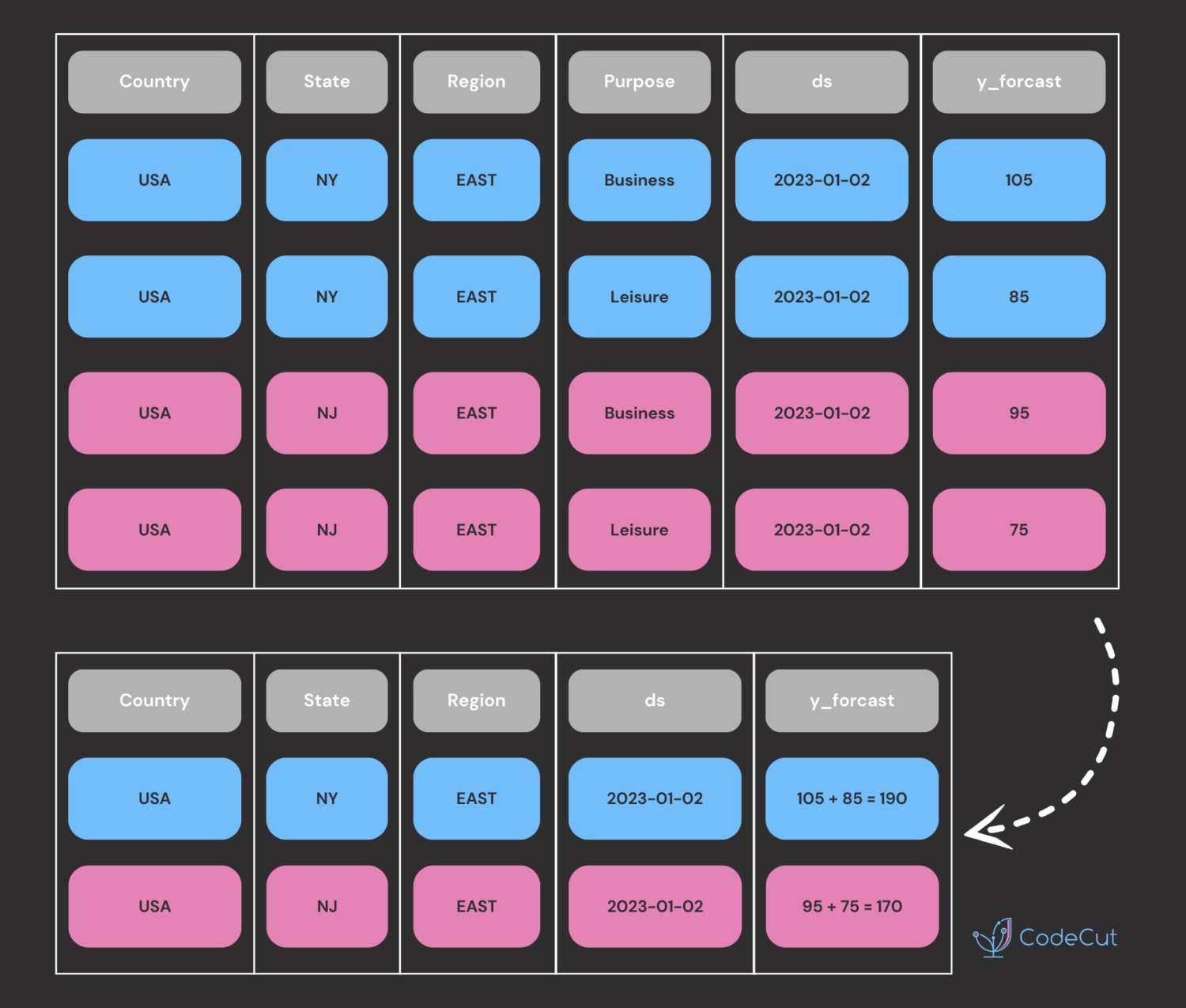
The bottom-up approach is a method where forecasts are initially created at the most granular level of a hierarchy and then aggregated up to higher levels. This approach ensures that detailed trends at lower levels are captured and accurately reflected in higher-level forecasts. It contrasts with top-down methods, which start with aggregate forecasts and distribute them downwards.

Steps in the Bottom-Up Approach

Forecast at the Lowest Level

First, forecasts are created at the most detailed level: Country, State, Region, Purpose. For example, the forecast for the next date might look like this:

CountryStateRegionPurposedsy_forecastUSANYEastBusiness2023-01-02105USANYEastLeisure2023-01-0285USANJEastBusiness2023-01-0295USANJEastLeisure2023-01-0275USACAWestBusiness2023-01-02125USACAWestLeisure2023-01-02115USANVWestBusiness2023-01-0265USANVWestLeisure2023-01-0255

Country, State, Purpose

Sum the forecasts for each Country, State, Purpose combination.

CountryStatePurposedsy_forecastUSANYBusiness2023-01-02105USANYLeisure2023-01-0285USANJBusiness2023-01-0295USANJLeisure2023-01-0275USACABusiness2023-01-02125USACALeisure2023-01-02115USANVBusiness2023-01-0265USANVLeisure2023-01-0255

Country, State, Region

Sum the forecasts for each Country, State, Region combination.

CountryStateRegiondsy_forecastUSANYEast2023-01-02190USANJEast2023-01-02170USACAWest2023-01-02240USANVWest2023-01-02120

Country, Purpose

Sum the forecasts for each Country, Purpose combination.

CountryPurposedsy_forecastUSABusiness2023-01-02390USALeisure2023-01-02330

Country

Sum the forecasts for the entire Country.

Countrydsy_forecastUSA2023-01-02720
Favorite

Hierarchical Forecasting in Python Read More »

Sliding Window Approach to Time Series Cross-Validation

Leave a Comment / Time Series / Khuyen Tran

Time series cross-validation evaluates a model’s predictive performance by training on past data and testing on subsequent time periods using a sliding window approach.

MLForecast offers an efficient and easy-to-use implementation of this technique.

To see how to implement time series cross-validation with MLForecast, let’s start reading a subset of the M4 Competition hourly dataset.

import pandas as pd
from utilsforecast.plotting import plot_series

Y_df = pd.read_csv("https://datasets-nixtla.s3.amazonaws.com/m4-hourly.csv").query(
"unique_id == 'H1'"
)
Y_df

unique_id ds y
0 H1 1 605.0
1 H1 2 586.0
2 H1 3 586.0
3 H1 4 559.0
4 H1 5 511.0
.. … … …
743 H1 744 785.0
744 H1 745 756.0
745 H1 746 719.0
746 H1 747 703.0
747 H1 748 659.0

[748 rows x 3 columns]

Plot the time series:

fig = plot_series(Y_df, plot_random=False, max_insample_length=24 * 14)
fig

Instantiate a new MLForecast object:

from mlforecast import MLForecast
from mlforecast.target_transforms import Differences
from sklearn.linear_model import LinearRegression

mlf = MLForecast(
models=[LinearRegression()],
freq=1,
target_transforms=[Differences([24])],
lags=range(1, 25),
)

Once the MLForecast object has been instantiated, we can use the cross_validation method.

For this particular example, we’ll use 3 windows of 24 hours.

# use 3 windows of 24 hours
cross_validation_df = mlf.cross_validation(
df=Y_df,
h=24,
n_windows=3,
)
cross_validation_df.head()

unique_id ds cutoff y LinearRegression
0 H1 677 676 691.0 676.726797
1 H1 678 676 618.0 559.559522
2 H1 679 676 563.0 549.167938
3 H1 680 676 529.0 505.930997
4 H1 681 676 504.0 481.981893

We’ll now plot the forecast for each cutoff period.

import matplotlib.pyplot as plt

def plot_cv(df, df_cv, last_n=24 * 14):
cutoffs = df_cv["cutoff"].unique()
fig, ax = plt.subplots(
nrows=len(cutoffs), ncols=1, figsize=(14, 6), gridspec_kw=dict(hspace=0.8)
)
for cutoff, axi in zip(cutoffs, ax.flat):
df.tail(last_n).set_index("ds").plot(ax=axi, y="y")
df_cv.query("cutoff == @cutoff").set_index("ds").plot(
ax=axi,
y="LinearRegression",
title=f"{cutoff=}",
)

plot_cv(Y_df, cross_validation_df)

Notice that in each cutoff period, we generated a forecast for the next 24 hours using only the data y before said period.

Link to MLForecast.

Run in Google Colab.
Favorite

Sliding Window Approach to Time Series Cross-Validation Read More »

Backtesting: Assess Trading Strategy Performance Effortlessly in Python

Leave a Comment / Testing, Time Series / Khuyen Tran

Evaluating trading strategies’ effectiveness is crucial for financial decision-making, but it’s challenging due to the complexities of historical data analysis and strategy testing.

Backtesting allows users to simulate trades based on historical data and visualize the outcomes through interactive plots in three lines of code.

To see how Backtesting works, let’s create our first strategy to backtest on these Google data, a simple moving average (MA) cross-over strategy.

from backtesting.test import GOOG

GOOG.tail()

Open High Low Close Volume
2013-02-25 802.3 808.41 790.49 790.77 2303900
2013-02-26 795.0 795.95 784.40 790.13 2202500
2013-02-27 794.8 804.75 791.11 799.78 2026100
2013-02-28 801.1 806.99 801.03 801.20 2265800
2013-03-01 797.8 807.14 796.15 806.19 2175400

import pandas as pd

def SMA(values, n):
"""
Return simple moving average of `values`, at
each step taking into account `n` previous values.
"""
return pd.Series(values).rolling(n).mean()

from backtesting import Strategy
from backtesting.lib import crossover

class SmaCross(Strategy):
# Define the two MA lags as *class variables*
# for later optimization
n1 = 10
n2 = 20

def init(self):
# Precompute the two moving averages
self.sma1 = self.I(SMA, self.data.Close, self.n1)
self.sma2 = self.I(SMA, self.data.Close, self.n2)

def next(self):
# If sma1 crosses above sma2, close any existing
# short trades, and buy the asset
if crossover(self.sma1, self.sma2):
self.position.close()
self.buy()

# Else, if sma1 crosses below sma2, close any existing
# long trades, and sell the asset
elif crossover(self.sma2, self.sma1):
self.position.close()
self.sell()

To assess the performance of our investment strategy, we will instantiate a Backtest object, using Google stock data as our asset of interest and incorporating the SmaCross strategy class. We’ll start with an initial cash balance of 10,000 units and set the broker’s commission to a realistic rate of 0.2%.

from backtesting import Backtest

bt = Backtest(GOOG, SmaCross, cash=10_000, commission=.002)
stats = bt.run()
stats

Start 2004-08-19 00:00:00
End 2013-03-01 00:00:00
Duration 3116 days 00:00:00
Exposure Time [%] 97.067039
Equity Final [$] 68221.96986
Equity Peak [$] 68991.21986
Return [%] 582.219699
Buy & Hold Return [%] 703.458242
Return (Ann.) [%] 25.266427
Volatility (Ann.) [%] 38.383008
Sharpe Ratio 0.658271
Sortino Ratio 1.288779
Calmar Ratio 0.763748
Max. Drawdown [%] -33.082172
Avg. Drawdown [%] -5.581506
Max. Drawdown Duration 688 days 00:00:00
Avg. Drawdown Duration 41 days 00:00:00
# Trades 94
Win Rate [%] 54.255319
Best Trade [%] 57.11931
Worst Trade [%] -16.629898
Avg. Trade [%] 2.074326
Max. Trade Duration 121 days 00:00:00
Avg. Trade Duration 33 days 00:00:00
Profit Factor 2.190805
Expectancy [%] 2.606294
SQN 1.990216
_strategy SmaCross
_equity_curve …
_trades Size EntryB…
dtype: object

Plot the outcomes:

bt.plot()

Link to Backtesting.

Run in Google Colab.
Favorite

Backtesting: Assess Trading Strategy Performance Effortlessly in Python Read More »

tsmoothie: Fast and Flexible Tool for Exponential Smoothing

Leave a Comment / Time Series / Khuyen Tran

Smoothing is useful for capturing the underlying pattern in time series data, especially for data with a strong trend or seasonal component.

The tsmoothie library is a fast and efficient Python tool for performing time-series smoothing operations.

To see how tsmoothie works, let’s generate a single random walk time series of length 200 using the sim_randomwalk() function.

import numpy as np
import matplotlib.pyplot as plt
from tsmoothie.utils_func import sim_randomwalk
from tsmoothie.smoother import LowessSmoother

# generate a random walk of length 200
np.random.seed(123)
data = sim_randomwalk(n_series=1, timesteps=200, process_noise=10, measure_noise=30)

Next, create a LowessSmoother object with a smooth_fraction of 0.1 (i.e., 10% of the data points are used for local regression) and 1 iteration. We then apply the smoothing operation to the data using the smooth() method.

# operate smoothing
smoother = LowessSmoother(smooth_fraction=0.1, iterations=1)
smoother.smooth(data)

After smoothing the data, we use the get_intervals() method of the LowessSmoother object to calculate the lower and upper bounds of the prediction interval for the smoothed time series.

# generate intervals
low, up = smoother.get_intervals("prediction_interval")

Finally, we plot the smoothed time series (as a blue line), and the prediction interval (as a shaded region) using matplotlib.

# plot the smoothed time series with intervals
plt.figure(figsize=(10, 5))

plt.plot(smoother.smooth_data[0], linewidth=3, color="blue")
plt.plot(smoother.data[0], ".k")
plt.title(f"timeseries")
plt.xlabel("time")

plt.fill_between(range(len(smoother.data[0])), low[0], up[0], alpha=0.3)

This graph effectively highlights the trend and seasonal components present in the time series data through the use of a smoothed representation.

Link to tsmoothie.

Run in Google Colab.
Favorite

tsmoothie: Fast and Flexible Tool for Exponential Smoothing Read More »

Beyond Point Estimates: Leverage Prediction Intervals for Robust Forecasting

Leave a Comment / Time Series / Khuyen Tran

Generating a forecast typically produces a single-point estimate, which does not reflect the uncertainty associated with the prediction.

To quantify this uncertainty, we need prediction intervals – a range of values the forecast can take with a given probability. MLForecast allows you to train sklearn models to generate both point forecasts and prediction intervals.

To demonstrate this, let’s consider the following example:

import pandas as pd
from utilsforecast.plotting import plot_series

train = pd.read_csv("https://auto-arima-results.s3.amazonaws.com/M4-Hourly.csv")
test = pd.read_csv("https://auto-arima-results.s3.amazonaws.com/M4-Hourly-test.csv")
train.head()
"""
unique_id ds y
0 H1 1 605.0
1 H1 2 586.0
2 H1 3 586.0
3 H1 4 559.0
4 H1 5 511.0
"""

We’ll only use the first series of the dataset.

n_series = 1
uids = train["unique_id"].unique()[:n_series]
train = train.query("unique_id in @uids")
test = test.query("unique_id in @uids")

Plot these series using the plot_series function from the utilsforecast library:

fig = plot_series(
df=train,
forecasts_df=test.rename(columns={"y": "y_test"}),
models=["y_test"],
palette="tab10",
)

fig.set_size_inches(8, 3)
fig

Train multiple models that follow the sklearn syntax:

from mlforecast import MLForecast
from mlforecast.target_transforms import Differences
from mlforecast.utils import PredictionIntervals
from sklearn.linear_model import LinearRegression
from sklearn.neighbors import KNeighborsRegressor

mlf = MLForecast(
models=[
LinearRegression(),
KNeighborsRegressor(),
],
freq=1,
target_transforms=[Differences([1])],
lags=[24 * (i + 1) for i in range(7)],
)

Apply the feature engineering and train the models:

mlf.fit(
data=train,
prediction_intervals=PredictionIntervals(n_windows=10, h=48),
)

Generate forecasts with prediction intervals:

# A list of floats with the confidence levels of the prediction intervals
levels = [50, 80, 95]

# Predict the next 48 hours
horizon = 48

# Generate forecasts with prediction intervals
forecasts = mlf.predict(h=horizon, level=levels)

Merge the test data with forecasts:

test_with_forecasts = test.merge(forecasts, how="left", on=["unique_id", "ds"])

Plot the point and the prediction intervals:

levels = [50, 80, 95]
fig = plot_series(
train,
test_with_forecasts,
plot_random=False,
models=["KNeighborsRegressor"],
level=levels,
max_insample_length=48,
palette='tab10',
)
fig.set_size_inches(8, 4)
fig

Link to MLForecast.

View in Google Colab.
Favorite

Beyond Point Estimates: Leverage Prediction Intervals for Robust Forecasting Read More »

Time Series

Extract Dates from Text with Datefinder

MLForecast: Automate External Feature Handling

Enhancing Predictive Models with Workalendar’s Holiday Handling

Avoiding Data Leakage in Time Series Analysis with TimeSeriesSplit

Pendulum: Python Datetimes Made Easy

Hierarchical Forecasting in Python

Sliding Window Approach to Time Series Cross-Validation

Backtesting: Assess Trading Strategy Performance Effortlessly in Python

tsmoothie: Fast and Flexible Tool for Exponential Smoothing

Beyond Point Estimates: Leverage Prediction Intervals for Robust Forecasting

Stay up-to-date with
data skills using
CodeCut

Drop a line

Get in touch

Follow Us on Social Media

Time Series

Stay up-to-date with data skills using CodeCut

Follow Us on Social Media

Work with Khuyen Tran

Work with Khuyen Tran

Stay up-to-date with
data skills using
CodeCut