In machine learning, we know that the performance of the loss function heavily depend on the hyperparameters of our model like the number of epochs, batch size, or dropout rate. A simple way to approach this is trying all the combinations of hyperparameters. But as their number grows, grid search quickly becomes slow and costly. Here’s a simple example using two hyperparameters:

best_score = float('-inf')
best_params = None

for epochs in [10, 50, 100]:
    for batch_size in [16, 32, 64]:
        model = train_model(epochs=epochs, batch_size=batch_size)
        score = evaluate_model(model)
        if score > best_score:
            best_score = score
            best_params = {'epochs': epochs, 'batch_size': batch_size}

print("Best score:", best_score)
print("Best params:", best_params)

Output:

Best score: 0.9149321112979663
Best params: {'epochs': 10, 'batch_size': 64}

A more efficient strategy is through Bayesian Optimization (BO). BO uses Gaussian Process Regression (GPR) to model our uncertainty and guides us where to search next in order to minimize our loss function.

In this article, you’ll learn how to apply GPR to improve your hyperparameter tuning strategy, in Python, using scikit-learn. We’ll walk through both theory and code, and show you how to build an optimization loop to find the best hyperparameter of your model.

Setup: Installing Libraries and Simulated Function

Let’s begin by installing and importing the necessary libraries.

import numpy as np
import matplotlib.pyplot as plt
from sklearn.gaussian_process import GaussianProcessRegressor
from sklearn.gaussian_process.kernels import Matern, WhiteKernel, ConstantKernel as C

We’ll also define a synthetic black-box function to optimize. In a data science project, the black-box function typically represents the entire training and evaluation pipeline of a machine learning model. Given a set of hyperparameters as input, it returns the corresponding error or loss value.

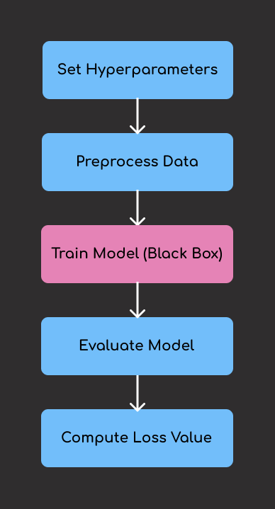
We call it a “black-box function” because, in real life, we don’t have an explicit mathematical formula for how hyperparameters affect the final performance. Instead, we can only train and observe the output error, which is expensive and time-consuming.

Here, we’re using a simplified synthetic function to emulate this process, but the principles we demonstrate apply equally to higher-dimensional hyperparameter spaces.

def black_box_function(x):
    return - (np.sin(3*x) + 0.5 * x)

Let’s visualize it:

# Generate 1000 evenly spaced values between 0 and 5.5
X = np.linspace(0, 5.5, 1000).reshape(-1, 1)

# Evaluate the black-box function on the generated values
y = black_box_function(X)

# Plot
plt.plot(X, y, "--", color="white")
plt.title("Black-box function")
plt.xlabel("x")
plt.ylabel("f(x)")

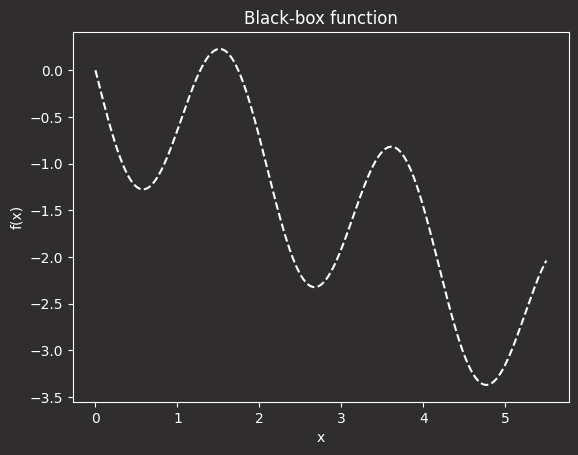
In the plot above:

• The x-axis represents a hyperparameter (e.g., learning rate, number of epochs).
• The y-axis shows the model’s performance (e.g,. error or loss).
• The function’s wavy shape reflects the unpredictable behavior of real-world performance across hyperparameters.
• The lowest point on the curve is the optimal hyperparameter, where the model performs best.

Key insights:

• Challenge: The true performance curve is unknown and costly to evaluate.
• Goal: Efficiently identify the best hyperparameter setting (i.e., the global minimum).
• Approach: Start with brute-force as a baseline, then introduce Gaussian Process-based Bayesian Optimization to search smarter and faster.

Brute force hyperparameter search

Imagine that x is your hyperparameter. You could try all the hyperparameters (multiple x values) and test which one is better:

# Create a grid of 100 evenly spaced values between 0 and 2
X_grid = np.linspace(0, 2, 100).reshape(-1, 1)

# Evaluate the black-box function at each point in the grid
y_grid = black_box_function(X_grid)

# Identify the input value that gives the maximum function output
x_best = X_grid[np.argmax(y_grid)]

Plot this approach:

plt.plot(X_grid, y_grid, '--', color='white', label="True function")
plt.scatter(X_grid, y_grid, c="#E583B6", label="Evaluated Points")
plt.scatter(x_best, black_box_function(x_best), c="#72BEFA", s=80, edgecolors="black", label="Best Point")

plt.title("Brute Force Search Over Full Range")
plt.xlabel("x")
plt.ylabel("f(x)")
plt.legend()

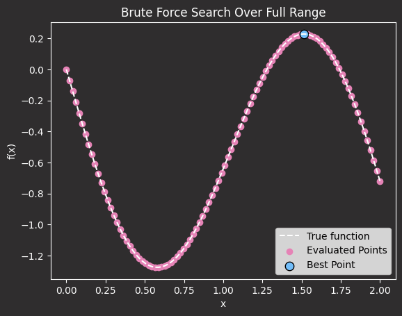
While this approach works, it is extremely inefficient and computationally expensive for real-world hyperparameter tuning.

For example, if x represents the number of epochs, evaluating 1000 different values means running 1000 separate training sessions, which could take days for large models.

Here’s a simple simulation of how costly that can be:

import numpy as np
import time

def train_model(epochs):
    time.sleep(0.1)  # Simulate a slow training step
    return - (np.sin(3 * epochs) + 0.5 * epochs)

search_space = np.linspace(0, 5, 1000)
results = []

start = time.time()
for x in search_space:
    loss = train_model(x)
    results.append((x, loss))
end = time.time()

print("Best x:", search_space[np.argmin([r[1] for r in results])])
print("Time taken:", round(end - start, 2), "seconds")

Output:

Best x: 4.76976976976977
Time taken: 103.8 seconds

Even in this small example, evaluating just 1000 points with a minimal 0.1-second delay already takes nearly two minutes, showing how quickly brute-force methods can become inefficient as the parameter space grows.

Introducing Gaussian Process Regression

A Gaussian Process is a probabilistic model that predicts not just the output of a function but also the uncertainty of that prediction by modeling a distribution over possible functions that fit the observed data.

To use a Gaussian Process, we need:

• A set of input-output pairs (initial evaluations of the function)
• A kernel function to define the similarity between input points
• A regression framework to fit the model and make predictions with uncertainty estimates

We begin by testing the model at a few chosen hyperparameter values and recording their results:

# Initial sample points (simulate prior evaluations)
X_sample = np.array([[1.0], [3.0], [5.5]])
y_sample = black_box_function(X_sample)

In a real-life scenario, if x is our hyperparameter, this would be like training a model using x = 30 epochs, x = 50 epochs, and x = 100 epochs to see how performance changes with that hyperparameter.

Next, define a kernel function to define the similarity between input points. We’ll use a flexible kernel that combines Matern and WhiteKernel to capture noise and complexity:

# Define the kernel
kernel = C(1.0) * Matern(length_scale=1.0, nu=2.5) + WhiteKernel(noise_level=1e-5)

# Create and fit the Gaussian Process model
gpr = GaussianProcessRegressor(kernel=kernel, alpha=0.0)
gpr.fit(X_sample, y_sample)

Next, let’s predict the function values across our domain and visualize the model’s mean prediction and uncertainty.

# Predict across the domain
mu, std = gpr.predict(X, return_std=True)

# Plot the result
plt.figure(figsize=(10, 5))
plt.plot(X, y, 'k--', label="True function")
plt.plot(X, mu, 'b-', label="GPR mean")
plt.fill_between(X.ravel(), mu - std, mu + std, alpha=0.3, label="Uncertainty")
plt.scatter(X_sample, y_sample, c='red', label="Samples")
plt.legend()
plt.title("Gaussian Process Fit")
plt.xlabel("x")
plt.ylabel("f(x)")
plt.show()

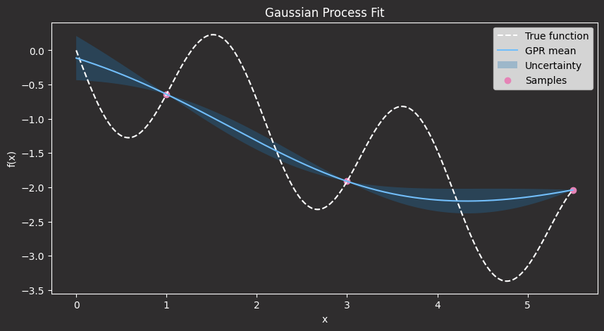
In the plot above:

• The black dashed line shows the true (unknown) function we aim to approximate.
• The red dots are the sample points we’ve already evaluated—our training data.
• The blue line is the Gaussian Process’s predicted mean of the function.
• The shaded blue area represents the model’s uncertainty—one standard deviation above and below the mean.

Notice how the uncertainty is low near the red dots, where we have data, and higher in regions where we haven’t sampled yet. This is one of the key strengths of GPR: it doesn’t just give us a prediction, but also tells us how confident it is in that prediction.

In the next step, we’ll use this uncertainty to guide where to sample next.

Bayesian Optimization Step

To pick the next hyperparameter to evaluate, we’ll define a quantity called Expected Improvement (EI). This quantity is our polar star, which will guide us to the next point to sample.

More specifically, EI is a statistical value that combines two things: the mean prediction of our Gaussian Process model (how good we think the function might be at a certain point) and the standard deviation (how uncertain we are about that prediction).

EI helps us decide where to sample next based on both potential performance and uncertainty:

• If the model predicts a low mean and has low uncertainty (confident that the point is good), EI will be high. It’s worth sampling.
• If uncertainty is high but the potential gain is large, EI will also be high. We should explore that point.
• If the model predicts a high mean and is confident (point is likely bad), EI will be low. It’s not worth evaluating.

As we will show below, the point with the largest EI will be selected as the next one to sample.

from scipy.stats import norm

def expected_improvement(X, X_sample, y_sample, model, xi=0.01):
    mu, std = model.predict(X, return_std=True)
    mu_sample_opt = np.min(y_sample)

    with np.errstate(divide='warn'):
        imp = mu_sample_opt - mu - xi  # because we are minimizing
        Z = imp / std
        ei = imp * norm.cdf(Z) + std * norm.pdf(Z)
        ei[std == 0.0] = 0.0

    return ei

Let’s compute and plot the EI over the search space:

ei = expected_improvement(X, X_sample, y_sample, gpr)

plt.figure(figsize=(10, 4))
plt.plot(X, ei, label="Expected Improvement")
plt.axvline(X[np.argmax(ei)], color='r', linestyle='--', label="Next sample point")
plt.title("Acquisition Function (Expected Improvement)")
plt.xlabel("x")
plt.ylabel("EI(x)")
plt.legend()
plt.show()

As we can see, we are correctly identifying the area where to sample, which is in the x in [3,5], as the area with the largest expected improvement. The maximum of EI will be the next point to sample. Once we sample that point, we can repeat the process in a loop, as shown in the next section.

Hypeparameter Search Loop

Let’s put everything in a loop that will search for the minimum of our function:

1. Fit Gaussian Process Regression (GPR) on a limited number of samples (input points and their loss values)
2. Compute the Expected Improvement (EI) on a larger number of sample points across the search space
3. Choose the next best point (the one with maximum EI)
4. Evaluate the function at the new point (compute loss at chosen point)
5. Retrain GPR with the new point and its loss value added to the training data
6. Repeat for a specified number of iterations

This is the code that implements the loop.

def bayesian_optimization(n_iter=10):
    # Initial data
    X_sample = np.array([[1.0], [2.5], [4.0]])
    y_sample = black_box_function(X_sample)

    for i in range(n_iter):
        gpr.fit(X_sample, y_sample)
        ei = expected_improvement(X, X_sample, y_sample, gpr)
        x_next = X[np.argmax(ei)].reshape(-1, 1)

        # Evaluate the function at the new point
        y_next = black_box_function(x_next)

        # Add the new sample to our dataset
        X_sample = np.vstack((X_sample, x_next))
        y_sample = np.append(y_sample, y_next)
    return X_sample, y_sample

And you can run it with:

X_opt, y_opt = bayesian_optimization(n_iter=10)

Final Visualization

We can see that with just 10 points (+3 initial samples), we have found the minimum.

# Plot final sampled points
plt.plot(X, black_box_function(X), 'k--', label="True function")
plt.scatter(X_opt, y_opt, c='red', label="Sampled Points")
plt.title("Bayesian Optimization with Gaussian Process")
plt.xlabel("x")
plt.ylabel("f(x)")
plt.legend()
plt.show()

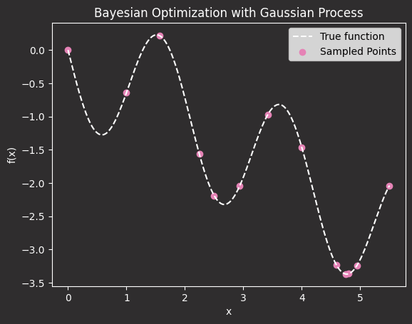
Et voilà. The minimum of your hyperparameter tuning process is found in only 10+3 steps.

This saves you from having to run hundreds of training sessions across different values of x, which is exactly what brute-force methods like grid search would require. In contrast, by using GPR, you only sample in the areas where you expect to find the minimum of your black-box function.

Summary: Benefits of Using Gaussian Processes for Tuning

Using Gaussian Processes for hyperparameter tuning offers:

• Fewer evaluations: Optimizes with less brute force.
• Smarter sampling: Focuses on promising regions.
• Uncertainty handling: Balances exploration and exploitation.
• Easy implementation: Works well with scikit-learn.

Adopting this technique leads to faster and more intelligent optimization, especially in scenarios where evaluating the loss function is expensive.