Beyond Point Estimates: Leverage Prediction Intervals for Robust Forecasting

Generating a forecast typically produces a single-point estimate, which does not reflect the uncertainty associated with the prediction.

To quantify this uncertainty, we need prediction intervals – a range of values the forecast can take with a given probability. MLForecast allows you to train sklearn models to generate both point forecasts and prediction intervals.

To demonstrate this, let’s consider the following example:

import pandas as pd
from utilsforecast.plotting import plot_series

train = pd.read_csv("https://auto-arima-results.s3.amazonaws.com/M4-Hourly.csv")
test = pd.read_csv("https://auto-arima-results.s3.amazonaws.com/M4-Hourly-test.csv")
train.head()
"""
  unique_id  ds      y
0        H1   1  605.0
1        H1   2  586.0
2        H1   3  586.0
3        H1   4  559.0
4        H1   5  511.0
"""

We’ll only use the first series of the dataset.

n_series = 1
uids = train["unique_id"].unique()[:n_series]  
train = train.query("unique_id in @uids")
test = test.query("unique_id in @uids")

Plot these series using the plot_series function from the utilsforecast library:

fig = plot_series(
    df=train,
    forecasts_df=test.rename(columns={"y": "y_test"}),
    models=["y_test"],
    palette="tab10",
)

fig.set_size_inches(8, 3)
fig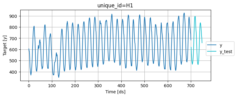

Train multiple models that follow the sklearn syntax:

from mlforecast import MLForecast
from mlforecast.target_transforms import Differences
from mlforecast.utils import PredictionIntervals
from sklearn.linear_model import LinearRegression
from sklearn.neighbors import KNeighborsRegressor

mlf = MLForecast(
    models=[
        LinearRegression(),
        KNeighborsRegressor(),
    ],
    freq=1,
    target_transforms=[Differences([1])],
    lags=[24 * (i + 1) for i in range(7)],
)

Apply the feature engineering and train the models:

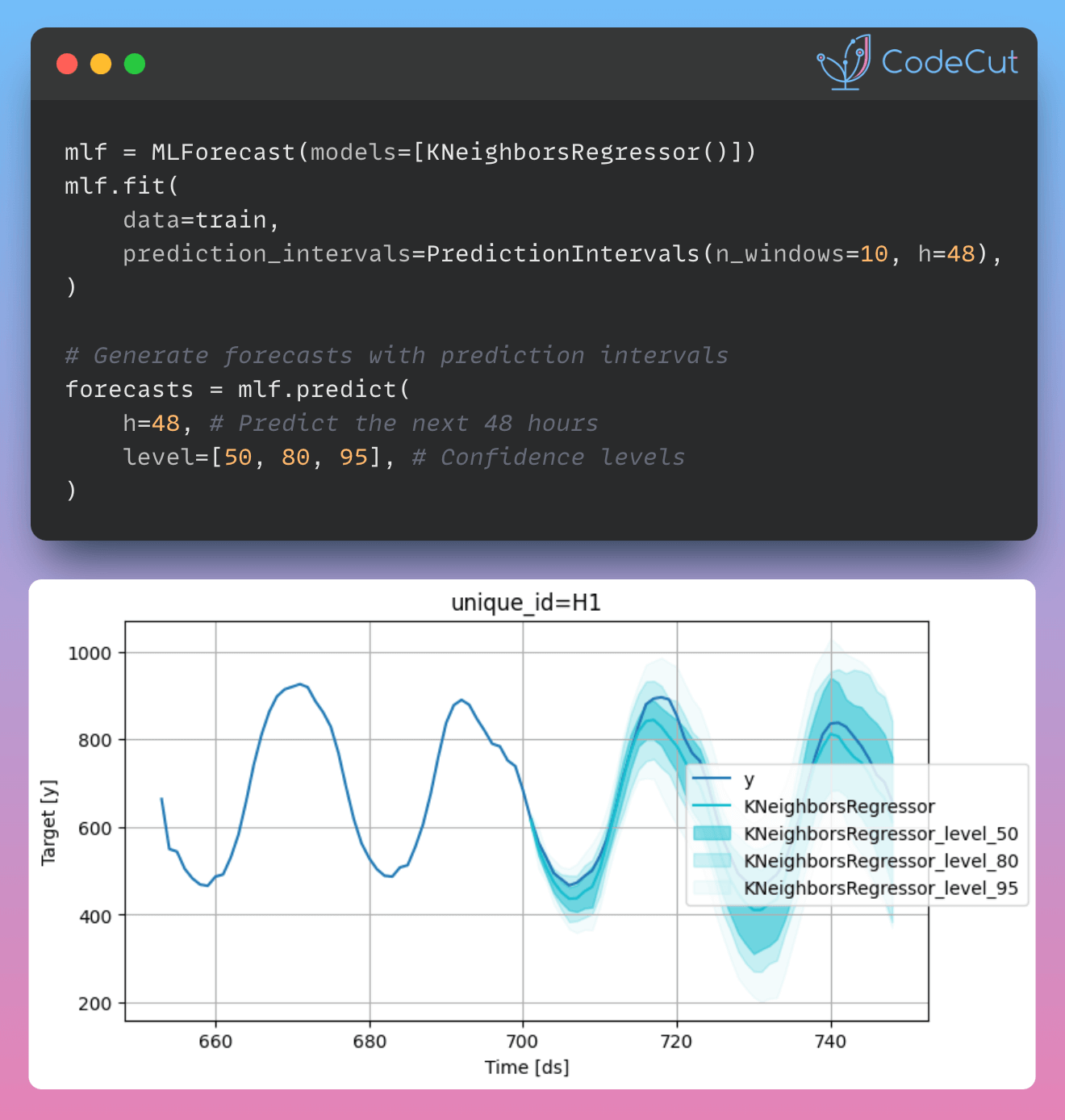
mlf.fit(
    data=train,
    prediction_intervals=PredictionIntervals(n_windows=10, h=48),
)

Generate forecasts with prediction intervals:

# A list of floats with the confidence levels of the prediction intervals
levels = [50, 80, 95]

# Predict the next 48 hours
horizon = 48

# Generate forecasts with prediction intervals
forecasts = mlf.predict(h=horizon, level=levels)

Merge the test data with forecasts:

test_with_forecasts = test.merge(forecasts, how="left", on=["unique_id", "ds"])

Plot the point and the prediction intervals:

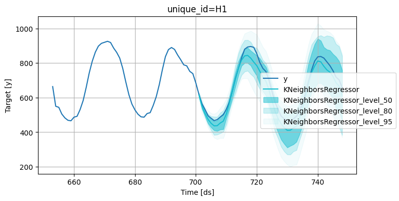
levels = [50, 80, 95]
fig = plot_series(
    train,
    test_with_forecasts,
    plot_random=False,
    models=["KNeighborsRegressor"],
    level=levels,
    max_insample_length=48,
    palette='tab10',
)
fig.set_size_inches(8, 4)
fig