Introduction

Are you tired of the overhead of setting up database servers just to run SQL queries? Do you struggle with pandas’ memory constraints when working with large datasets?

DuckDB provides a streamlined approach: as an embedded SQL database, it enables direct data querying without any server configuration. It significantly outperforms pandas in terms of both performance and memory efficiency, especially when handling complex operations like joins and aggregations on large datasets.

In this post, we’ll dive into some of the key features of DuckDB and how it can be used to supercharge your data science workflow.

What is DuckDB?

DuckDB is a fast, in-process SQL OLAP database optimized for analytics. DuckDB is a great tool for data scientists because of the following reasons:

1. Zero Configuration: No need to set up or maintain a separate database server
2. Memory Efficiency: Process large datasets without loading everything into memory
3. Familiar Interface: Use SQL syntax you already know, directly in Python
4. Performance: Faster than pandas for many operations, especially joins and aggregations
5. File Format Support: Direct querying of CSV, Parquet, and other file formats

To install DuckDB, run the following command:

pip install duckdb

In the next few sections, we’ll dive into some of the key features of DuckDB and how it can be used to supercharge your data science workflow.

Zero Configuration

SQL operations on DataFrames typically require setting up and maintaining separate database servers, adding complexity to analytical workflows.

For example, to perform a simple SQL operation on a DataFrame, you need to:

• Install and configure a database server (like PostgreSQL or MySQL)
• Ensure the database service is running before executing queries
• Set up database credentials
• Create a connection to the database
• Write the DataFrame to a PostgreSQL table

import pandas as pd
from sqlalchemy import create_engine


# Create sample data
sales = pd.DataFrame(
    {
        "product": ["A", "B", "C", "A", "B", "C"] * 2,
        "region": ["North", "South"] * 6,
        "amount": [100, 150, 200, 120, 180, 220, 110, 160, 210, 130, 170, 230],
        "date": pd.date_range("2024-01-01", periods=12),
    }
)


# Create a connection to PostgreSQL
engine = create_engine("postgresql://postgres:postgres@localhost:5432/postgres")

# Write the DataFrame to a PostgreSQL table
sales.to_sql("sales", engine, if_exists="replace", index=False)

# Execute SQL query against the PostgreSQL database
with engine.connect() as conn:
    result = pd.read_sql("SELECT product, region, amount FROM sales", conn)

print(result.head(5))

  product region  amount
0       A  North     100
1       B  South     150
2       C  North     200
3       A  South     120
4       B  North     180

This overhead can be particularly cumbersome when you just want to perform quick SQL operations on your data.

DuckDB simplifies this process by providing direct SQL operations on DataFrames without server setup:

import duckdb

# Direct SQL operations on DataFrame - no server needed
result = duckdb.sql("SELECT product, region, amount FROM sales").df()

print(result.head(5))

product region  amount
0       A  North     100
1       B  South     150
2       C  North     200
3       A  South     120
4       B  North     180

Integrate Seamlessly with pandas and Polars

Have you ever wanted to leverage SQL’s power while working with your favorite data manipulation libraries such as pandas and Polars?

DuckDB makes it seamless to query pandas and Polars DataFrames via the duckdb.sql function.

import duckdb
import pandas as pd
import polars as pl

pd_df = pd.DataFrame({"a": [1, 2, 3], "b": [4, 5, 6]})

pl_df = pl.DataFrame({"a": [1, 2, 3], "b": [4, 5, 6]})

duckdb.sql("SELECT * FROM pd_df").df()
duckdb.sql("SELECT * FROM pl_df").df()

DuckDB’s integration with pandas and Polars lets you combine the strengths of each tool. For example, you can:

• Use pandas for data cleaning and feature engineering
• Use DuckDB for complex aggregations and complex queries

import pandas as pd
import duckdb

# Use pandas for data cleaning and feature engineering
sales['month'] = sales['date'].dt.month
sales['is_high_value'] = sales['amount'] > 150
print("Sales after feature engineering:")
print(sales.head())

Sales after feature engineering:
  product region  amount       date  month  is_high_value
0       A  North     100 2024-01-01      1          False
1       B  South     150 2024-01-02      1          False
2       C  North     200 2024-01-03      1           True
3       A  South     120 2024-01-04      1          False
4       B  North     180 2024-01-05      1           True

# Use DuckDB for complex aggregations
analysis = duckdb.sql("""
    SELECT 
        product,
        region,
        COUNT(*) as total_sales,
        AVG(amount) as avg_amount,
        SUM(CASE WHEN is_high_value THEN 1 ELSE 0 END) as high_value_sales
    FROM sales
    GROUP BY product, region
    ORDER BY avg_amount DESC
""").df()

print("Sales analysis by product and region:")
print(analysis)

Sales analysis by product and region:
  product region  total_sales  avg_amount  high_value_sales
0       C  South            2       225.0               2.0
1       C  North            2       205.0               2.0
2       B  North            2       175.0               2.0
3       B  South            2       155.0               1.0
4       A  South            2       125.0               0.0
5       A  North            2       105.0               0.0

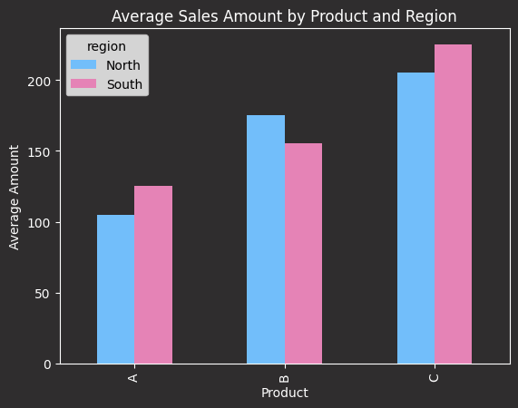
# Use pandas for visualization
from utils import apply_codecut_style
import matplotlib.pyplot as plt

# Create a simple bar plot
ax = analysis.pivot_table(
    values="avg_amount", index="product", columns="region"
).plot(kind="bar", color=["#72BEFA", "#E583B6"])

ax.set_title("Average Sales Amount by Product and Region")
ax.set_xlabel("Product")
ax.set_ylabel("Average Amount")
apply_codecut_style(ax)

Memory Efficiency

A major drawback of pandas is its in-memory processing requirement. It must load complete datasets into RAM before any operations can begin, which can trigger out-of-memory errors when analyzing large datasets.

To demonstrate this, we’ll create a large dataset (1 million rows) and save it as a CSV file.

import pandas as pd
import numpy as np
import time
import duckdb

# Create sample datasets
n_rows = 1_000_000

# Customers dataset
customers = pd.DataFrame({
    'customer_id': range(n_rows),
    'name': [f'Customer_{i}' for i in range(n_rows)],
    'region': np.random.choice(['North', 'South', 'East', 'West'], n_rows),
    'segment': np.random.choice(['A', 'B', 'C'], n_rows)
})

# Save to Parquet
customers.to_csv('data/customers.csv', index=False)

To filter for customers in the ‘North’ region, pandas loads all 1 million customer records into RAM, even though we only need a subset of the data.

import pandas as pd

# Load CSV file
df = pd.read_csv('data/customers.csv')

# Filter the data
result = df[df['region'] == 'North']
print(result.head(5))

customer_id         name region segment
9             9   Customer_9  North       B
11           11  Customer_11  North       C
17           17  Customer_17  North       B
19           19  Customer_19  North       C
23           23  Customer_23  North       B

Unlike pandas which loads the entire dataset into memory, DuckDB uses a columnar storage format and query optimization to only process the rows where region = 'North'.

import duckdb

# Query a CSV file directly
result = duckdb.sql("""
    SELECT *
    FROM 'data/customers.csv'
    WHERE region = 'North'
""").df()
print(result.head(5))

customer_id         name region segment
9             9   Customer_9  North       B
11           11  Customer_11  North       C
17           17  Customer_17  North       B
19           19  Customer_19  North       C
23           23  Customer_23  North       B

This selective loading approach significantly reduces memory usage, especially when working with large datasets.

Fast Performance

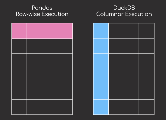
While pandas processes data sequentially row-by-row, DuckDB uses a vectorized execution engine that processes data in parallel chunks. This architectural difference enables DuckDB to significantly outperform pandas, especially for computationally intensive operations like aggregations and joins.

Let’s compare the performance of pandas and DuckDB for aggregations on a million rows of data.

import time

# Pandas aggregation
start_time = time.time()
pandas_agg = customers.groupby(['region', 'segment']).size().reset_index(name='count')
pandas_time = time.time() - start_time

# DuckDB aggregation
start_time = time.time()
duckdb_agg = duckdb.sql("""
    SELECT region, segment, COUNT(*) as count FROM customers GROUP BY region, segment
""").df()
duckdb_time = time.time() - start_time

# Print the results
print(f"Pandas aggregation time: {pandas_time:.2f} seconds")
print(f"DuckDB aggregation time: {duckdb_time:.2f} seconds")
print(f"Speedup: {pandas_time/duckdb_time:.1f}x")

Pandas aggregation time: 0.13 seconds
DuckDB aggregation time: 0.02 seconds
Speedup: 8.7x

We can see that DuckDB is much faster than pandas for aggregations. The performance difference becomes even more pronounced when working with larger datasets.

Streamlined File Reading

Automatic Parsing of CSV Files

When working with CSV files that have non-standard delimiters, you need to specify key parameters like delimiter and header with pandas to avoid parsing errors.

To demonstrate this, let’s create a CSV file with a custom delimiter and header.

import pandas as pd

# Example CSV content with a custom delimiter
csv_content = """FlightDate|UniqueCarrier|OriginCityName|DestCityName
1988-01-01|AA|New York, NY|Los Angeles, CA
1988-01-02|AA|New York, NY|Los Angeles, CA
1988-01-03|AA|New York, NY|Los Angeles, CA
"""

## Writing the CSV content to a file
with open("data/flight_data.csv", "w") as f:
    f.write(csv_content)

## Reading the CSV file with pandas without specifying the delimiter
df = pd.read_csv("data/flight_data.csv")
print(df)

                                      FlightDate|UniqueCarrier|OriginCityName|DestCityName
1988-01-01|AA|New York NY|Los Angeles                                                 CA  
1988-01-02|AA|New York NY|Los Angeles                                                 CA  
1988-01-03|AA|New York NY|Los Angeles    

The output shows that pandas assumed the default delimiter (,) and incorrectly parsed the data into a single column.

DuckDB’s read_csv feature automatically detects the structure of the CSV file, including delimiters, headers, and column types.

import duckdb

## Use DuckDB to automatically detect and read the CSV structure
result = duckdb.query("SELECT * FROM read_csv('data/flight_data.csv')").to_df()
print(result)

FlightDate UniqueCarrier OriginCityName     DestCityName
0 1988-01-01            AA   New York, NY  Los Angeles, CA
1 1988-01-02            AA   New York, NY  Los Angeles, CA
2 1988-01-03            AA   New York, NY  Los Angeles, CA

The output shows that DuckDB automatically detected the correct delimiter (|) and correctly parsed the data into columns.

Automatic Flattening of Nested Parquet Files

When working with large, nested Parquet files, you typically need to pre-process the data to flatten nested structures or write complex extraction scripts, which adds time and complexity to your workflow.

To demonstrate this, let’s create a nested dataset and save it as a Parquet file.

import pandas as pd

# Create a nested dataset and save it as a Parquet file
data = {
    "id": [1, 2],
    "details": [{"name": "Alice", "age": 25}, {"name": "Bob", "age": 30}],
}

## Convert to a DataFrame
df = pd.DataFrame(data)

# Save as a nested Parquet file
df.to_parquet("data/customers.parquet")

To flatten the nested data with pandas, you need to create a new DataFrame with the flattened structure.

## Read the DataFrame from Parquet file
df = pd.read_parquet("data/customers.parquet")

# Create a new DataFrame with the flattened structure
flat_df = pd.DataFrame(
    {
        "id": df["id"],
        "name": [detail["name"] for detail in df["details"]],
        "age": [detail["age"] for detail in df["details"]],
    }
)

print(flat_df)

id   name  age
0   1  Alice   25
1   2    Bob   30

DuckDB allows you to query nested Parquet files directly using SQL without needing to flatten or preprocess the data. This is much more efficient than pandas.

import duckdb

## Query the nested Parquet file directly
query_result = duckdb.query(
    """
    SELECT
        id,
        details.name AS name,
        details.age AS age
    FROM read_parquet('data/customers.parquet')
"""
).to_df()

print(query_result)

id   name  age
0   1  Alice   25
1   2    Bob   30

In this example:

• read_parquet('customers.parquet') reads the nested Parquet file.
• SQL syntax allows you to access nested fields using dot notation (e.g., details.name).

The output is a flattened representation of the nested data, directly queried from the Parquet file without additional preprocessing.

Automatic Flattening of Nested JSON Files

When working with JSON files that have nested structures, you need to normalize the data with pandas to access nested fields.

To demonstrate this, let’s create a nested JSON file.

import pandas as pd
import numpy as np
import json

# Create sample JSON data
n_rows = 5

# Generate nested JSON data
data = []
for i in range(n_rows):
    record = {
        "user_id": i,
        "profile": {"name": f"User_{i}", "active": np.random.choice([True, False])},
    }
    data.append(record)

# Save as JSON file
with open("data/users.json", "w") as f:
    json.dump(data, f, default=str)

This is a sample of the JSON file:

[{'profile': {'active': 'False', 'name': 'User_0'}, 'user_id': 0},
 {'profile': {'active': 'True', 'name': 'User_1'}, 'user_id': 1},
 {'profile': {'active': 'False', 'name': 'User_2'}, 'user_id': 2},
 {'profile': {'active': 'True', 'name': 'User_3'}, 'user_id': 3},
 {'profile': {'active': 'False', 'name': 'User_4'}, 'user_id': 4}]

When working with nested JSON data in pandas, you’ll need to use pd.json_normalize to flatten the nested structure. This step is required to access nested fields in a tabular format.

# Load JSON with pandas
import pandas as pd

df_normalized = pd.json_normalize(
    data,
    meta=["user_id", ["profile", "name"], ["profile", "active"]],
)

print("Normalized data:")
print(df_normalized)

Normalized data:
   user_id profile.name profile.active
0        0       User_0          False
1        1       User_1           True
2        2       User_2          False
3        3       User_3           True
4        4       User_4          False

With DuckDB, you can query each nested field directly with the syntax field_name.nested_field_name.

import duckdb

# Query JSON directly
result = duckdb.sql(
    """
    SELECT
        user_id,
        profile.name,
        profile.active
    FROM read_json('data/users.json')
"""
).df()

print("JSON query results:")
print(result)

JSON query results:
   user_id    name active
0        0  User_0  False
1        1  User_1   True
2        2  User_2  False
3        3  User_3   True
4        4  User_4  False

Reading Multiple Files

Reading Multiple Files from a Directory

It can be complicated to read multiple files from a folder with pandas.

Let’s say we have two CSV files in the data/sales directory. One containing January sales data and another with February sales data. Our goal is to combine both files into a single DataFrame for analysis.

from pathlib import Path

import pandas as pd

# Create example dataframe for first file
df1 = pd.DataFrame(
    {
        "Date": ["2023-01-01", "2023-01-02", "2023-01-03"],
        "Product": ["Laptop", "Phone", "Tablet"],
        "Sales": [1200, 800, 600],
    }
)

# Create example dataframe for second file
df2 = pd.DataFrame(
    {
        "Date": ["2023-02-01", "2023-02-02", "2023-02-03"],
        "Product": ["Laptop", "Monitor", "Mouse"],
        "Sales": [1500, 400, 50],
    }
)

Path("data/sales").mkdir(parents=True, exist_ok=True)
df1.to_csv("data/sales/jan.csv", index=False)
df2.to_csv("data/sales/feb.csv", index=False)

With pandas, you need to read each file separately then concatenate them.

import pandas as pd
import duckdb

# Read each file separately
df1 = pd.read_csv("data/sales/jan.csv")
df2 = pd.read_csv("data/sales/feb.csv")

# Concatenate the two DataFrames
df = pd.concat([df1, df2])
print(df.sort_values(by="Date"))

Date  Product  Sales
0  2023-01-01   Laptop   1200
1  2023-01-02    Phone    800
2  2023-01-03   Tablet    600
0  2023-02-01   Laptop   1500
1  2023-02-02  Monitor    400
2  2023-02-03    Mouse     50

With DuckDB, you can read all the files in the data/sales folder at once.

import duckdb

## Read and analyze all CSV files at once
result = duckdb.sql(
    """
    SELECT *
    FROM 'data/sales/*.csv'
"""
).df()
print(result.sort_values(by="Date"))

Date  Product  Sales
3 2023-01-01   Laptop   1200
4 2023-01-02    Phone    800
5 2023-01-03   Tablet    600
0 2023-02-01   Laptop   1500
1 2023-02-02  Monitor    400
2 2023-02-03    Mouse     50

The result is a single DataFrame with all the data from both files.

Read From Multiple Sources

DuckDB allows you to read data from multiple sources in a single query, making it easier to combine data from different sources.

To demonstrate, let’s create some sample data in two different formats: a CSV file and a Parquet file.

import pandas as pd
import numpy as np
import json

# Create sample data in different formats
n_rows = 5

# 1. Create a CSV file with customer data
customers = pd.DataFrame(
    {
        "customer_id": range(n_rows),
        "region": np.random.choice(["North", "South", "East", "West"], n_rows),
    }
)
customers.to_csv("data/customers.csv", index=False)

# 2. Create a Parquet file with order data
orders = pd.DataFrame(
    {
        "order_id": range(n_rows),
        "customer_id": np.random.randint(0, n_rows, n_rows),
        "amount": np.random.normal(100, 30, n_rows),
    }
)
orders.to_parquet("data/orders.parquet")

Now let’s query across all these sources in a single query.

import duckdb

# Query combining data from CSV and Parquet
result = duckdb.sql(
    """
    SELECT
        c.region,
        COUNT(DISTINCT c.customer_id) as unique_customers,
        AVG(o.amount) as avg_order_amount,
        SUM(o.amount) as total_revenue
    FROM 'data/customers.csv' c
    JOIN 'data/orders.parquet' o
        ON c.customer_id = o.customer_id
    GROUP BY c.region
    ORDER BY total_revenue DESC
"""
).df()

print("Sales Analysis by Region:")
print(result)

The result is a single DataFrame with the sales data from both files.

Parameterized Queries

When working with databases, you often need to run similar queries with different parameters. For instance, you might want to filter a table using various criteria.

Let’s demonstrate this by creating an accounts table and inserting some sample data.

import duckdb

# Create a new database file
conn = duckdb.connect("data/bank.db")

# Create accounts table
conn.sql(
    """
    CREATE TABLE accounts (account_id INTEGER, name VARCHAR, balance DECIMAL(10,2))
"""
)

# Insert sample accounts
conn.sql(
    """
    INSERT INTO accounts VALUES(1, 'Alice', 1000.00), (2, 'Bob', 500.00), (3, 'Charlie', 750.00)
"""
)

Now, you might want to search for accounts by different names or filter by different balance thresholds and reuse the same query multiple times.

You can do this by using f-strings to pass parameters to your queries.

import duckdb

# Open a connection
conn = duckdb.connect("data/bank.db")

name_1 = "A"
balance_1 = 100

name_2 = "C"
balance_2 = 200

# Execute a query with parameters
result_1 = conn.sql(
    f"SELECT * FROM accounts WHERE starts_with(name, '{name_1}') AND balance > {balance_1}"
).df()

result_2 = conn.sql(
    f"SELECT * FROM accounts WHERE starts_with(name, '{name_2}') AND balance > {balance_2}"
).df()

print(f"result_1:\n{result_1}")
print(f"result_2:\n{result_2}")

While this works, it’s not a good idea as it can lead to SQL injection attacks.

DuckDB provides safer ways to add parameters to your queries with parameterized queries.

Parameterized queries allow you to pass values as arguments to your queries using the execute method and the ? placeholder.

result_1 = conn.execute(
    "SELECT * FROM accounts WHERE starts_with(name, ?) AND balance > ?",
    (name_1, balance_1),
).df()

result_2 = conn.execute(
    "SELECT * FROM accounts WHERE starts_with(name, ?) AND balance > ?",
    (name_2, balance_2),
).df()

print(f"result_1:\n{result_1}")
print(f"result_2:\n{result_2}")

ACID Transactions

DuckDB supports ACID transactions on your data. Here are the properties of ACID transactions:

• Atomicity: The transaction either completes entirely or has no effect at all. If any operation fails, all changes are rolled back.
• Consistency: The database maintains valid data by enforcing all rules and constraints throughout the transaction.
• Isolation: Transactions run independently without interfering with each other
• Durability: Committed changes are permanent and survive system failures

Let’s demonstrate ACID properties with a bank transfer:

import duckdb

# Open a connection
conn = duckdb.connect("data/bank.db")


def transfer_money(from_account, to_account, amount):
    # Begin transaction
    conn.sql("BEGIN TRANSACTION")

    # Check balance
    balance = conn.execute(
        "SELECT balance FROM accounts WHERE account_id = ?", (from_account,)
    ).fetchone()[0]

    if balance >= amount:
        # Deduct money
        conn.execute(
            "UPDATE accounts SET balance = balance - ? WHERE account_id = ?",
            (amount, from_account),
        )

        # Add money
        conn.execute(
            "UPDATE accounts SET balance = balance + ? WHERE account_id = ?",
            (amount, to_account),
        )

        # Commit transaction
        conn.sql("COMMIT")
    else:
        # Rollback transaction
        conn.sql("ROLLBACK")
        print(f"Insufficient funds: {balance}")

In the code above:

• BEGIN TRANSACTION starts a transaction block where all SQL statements are grouped together as one unit. Changes remain hidden until committed.

• COMMIT finalizes a transaction by permanently saving all changes made within the transaction block to the database. After a commit, the changes become visible to other transactions and cannot be rolled back.

• ROLLBACK cancels all changes made within the current transaction block and restores the database to its state before the transaction began. This is useful for handling errors or invalid operations, ensuring data consistency.

Let’s try this out with a valid transfer and an invalid transfer.

# Show initial balances
print("Initial balances:")
print(conn.sql("SELECT * FROM accounts").df())

# Perform a valid transfer
print("\nPerforming valid transfer of $200 from Alice to Bob:")
transfer_money(1, 2, 200)

# Show balances after valid transfer
print("\nBalances after valid transfer:")
print(conn.sql("SELECT * FROM accounts").df())

# Attempt an invalid transfer (insufficient funds)
print("\nAttempting invalid transfer of $1000 from Bob to Charlie:")
transfer_money(2, 3, 1000)

# Show balances after failed transfer (should be unchanged)
print("\nBalances after failed transfer (should be unchanged):")
print(conn.sql("SELECT * FROM accounts").df())

This bank transfer example demonstrates all ACID properties:

• Atomicity: If the transfer fails (e.g., insufficient funds), both the deduction from Alice’s account and addition to Bob’s account are rolled back. The money is never lost in transit.
• Consistency: The total balance of $1500 remains constant across all accounts. When Alice transfers $200 to Bob, her balance decreases by $200 and Bob’s increases by $200.
• Isolation: If multiple transfers happen simultaneously (e.g., Alice sending money to Bob while Charlie sends money to Alice), they won’t interfere with each other. Each sees the correct account balances.
• Durability: After the successful $200 transfer from Alice to Bob, their new balances ($300 and $700) are permanently saved, even if the system crashes.

This makes DuckDB suitable for:

• Financial applications
• Data integrity critical operations
• Concurrent data processing
• Reliable data updates

Extensible

DuckDB offers a rich set of extensions that can be used to add additional functionality to the database.

To demonstrate the full-text search extension, let’s create a table with articles and insert some sample data.

import duckdb

# Create a connection
conn = duckdb.connect('data/articles.db')

# Create a table with articles
conn.sql("""
    CREATE OR REPLACE TABLE articles (
        article_id VARCHAR,
        title VARCHAR,
        content VARCHAR,
        publish_date DATE
    )
""")

# Insert sample articles
conn.sql("""
    INSERT INTO articles VALUES
        ('art1', 'Introduction to DuckDB',
         'DuckDB is an embedded analytical database that supports SQL queries on local files.',
         '2024-01-15'),
        ('art2', 'Working with Large Datasets',
         'Learn how to efficiently process large datasets using DuckDB and its powerful features.',
         '2024-02-01'),
        ('art3', 'SQL Performance Tips',
         'Optimize your SQL queries for better performance in analytical workloads.',
         '2024-02-15')
""")

Now let’s use the full-text search capabilities. First, we need to create a full-text search index on the articles table using the PRAGMA create_fts_index function. This function takes:

• input_table: The name of the table to create the full-text search index on.
• input_id: The name of the column to use as the unique identifier for each row.
• *input_values: The names of the columns to include in the full-text search index.

conn.sql("""
    PRAGMA create_fts_index('articles', 'article_id', 'title', 'content')
""")

Then, we can search for articles about DuckDB by using the fts_main_articles.match_bm25 function. This function takes:

• input_id: The name of the column to use as the unique identifier for each row.
• query_string: The search query to match against the full-text search index.
• fields: The names of the columns to include in the full-text search index.

results = conn.sql("""
    SELECT article_id, title, content, score
    FROM (
        SELECT *, fts_main_articles.match_bm25(article_id, 'DuckDB', fields := 'title,content') AS score
        FROM articles
    ) sq
    WHERE score IS NOT NULL
    ORDER BY score DESC
""").df()

print("Articles about DuckDB:")
print(results)

Articles about DuckDB:
  article_id                        title  \
0       art1       Introduction to DuckDB   
1       art2  Working with Large Datasets   

                                             content     score  
0  DuckDB is an embedded analytical database that...  0.275663  
1  Learn how to efficiently process large dataset...  0.198871

The result is a DataFrame with the articles that include the word “DuckDB” in the title or content.

View the full list of extensions on DuckDB’s extensions page.

Key Takeaways

DuckDB empowers data scientists with several key advantages:

• Zero-configuration SQL querying without database server setup
• Seamless integration with pandas and Polars DataFrames
• Efficient memory management for large-scale data processing
• High-performance execution of complex operations including joins and aggregations
• ACID transaction support ensuring data integrity
• Extensible architecture with a comprehensive extension ecosystem

With DuckDB, you can unlock a new level of productivity and efficiency in your data analysis workflows.