In complex datasets, forecasts at detailed levels (e.g., regions, products) should align with higher-level forecasts (e.g., countries, categories). Inconsistent forecasts can lead to poor decisions.
Hierarchical forecasting ensures forecasts are consistent across all levels to reconcile and match forecasts from lower to higher levels.
HierarchicalForecast from Nixtla is an open-source library that provides tools and methods for creating and reconciling hierarchical forecasts
For illustrative purposes, consider a sales dataset with the following columns:
- Country: The country where the sales occurred.
- Region: The region within the country.
- State: The state within the region.
- Purpose: The purpose of the sale (e.g., Business, Leisure).
- ds: The date of the sale.
- y: The sales amount.
import numpy as np
import pandas as pd

Y_df = pd.read_csv('https://raw.githubusercontent.com/Nixtla/transfer-learning-time-series/main/datasets/tourism.csv')
Y_df = Y_df.rename({'Trips': 'y', 'Quarter': 'ds'}, axis=1)
Y_df.insert(0, 'Country', 'Australia')
Y_df = Y_df[['Country', 'State', 'Region', 'Purpose', 'ds', 'y']]
Y_df['ds'] = Y_df['ds'].str.replace(r'(\d+) (Q\d)', r'\1-\2', regex=True)
Y_df['ds'] = pd.to_datetime(Y_df['ds'])
Y_df.head()| Country | State | Region | Purpose | ds | y |
|---|---|---|---|---|---|
| Australia | South Australia | Adelaide | Business | 1998-01-01 | 135.077690 |
| Australia | South Australia | Adelaide | Business | 1998-04-01 | 109.987316 |
| Australia | South Australia | Adelaide | Business | 1998-07-01 | 166.034687 |
| Australia | South Australia | Adelaide | Business | 1998-10-01 | 127.160464 |
| Australia | South Australia | Adelaide | Business | 1999-01-01 | 137.448533 |
The dataset can be grouped in the following non-strictly hierarchical structure:
- Country
- Country, State
- Country, Purpose
- Country, State, Region
- Country, State, Purpose
- Country, State, Region, Purpose
spec = [
    ['Country'],
    ['Country', 'State'],
    ['Country', 'Purpose'],
    ['Country', 'State', 'Region'],
    ['Country', 'State', 'Purpose'],
    ['Country', 'State', 'Region', 'Purpose']
]
Using the aggregate function from HierarchicalForecast we can get the full set of time series.
from hierarchicalforecast.utils import aggregate

Y_df, S_df, tags = aggregate(Y_df, spec)
Y_df = Y_df.reset_index()
Y_df.sample(10)| unique_id | ds | y |
|---|---|---|
| 12251 | Australia/New South Wales/Outback NSW/Business | 2000-10-01 |
| 33131 | Australia/Western Australia/Australia’s North | 2000-10-01 |
| 22034 | Australia/South Australia/Fleurieu Peninsula/Other | 2006-07-01 |
| 31119 | Australia/Victoria/Phillip Island/Visiting | 2017-10-01 |
| 7671 | Australia/New South Wales/Other | 2015-10-01 |
| 18339 | Australia/Queensland/Mackay/Business | 2002-10-01 |
| 23043 | Australia/South Australia/Limestone Coast/Visiting | 1998-10-01 |
| 22129 | Australia/South Australia/Fleurieu Peninsula/Visiting | 2010-04-01 |
| 11349 | Australia/New South Wales/Hunter/Business | 2015-04-01 |
| 16599 | Australia/Queensland/Brisbane/Other | 2007-10-01 |
Get all the distinct ‘Country/Purpose’ combinations present in the dataset:
tags['Country/Purpose']array(['Australia/Business', 'Australia/Holiday', 'Australia/Other',
'Australia/Visiting'], dtype=object)We use the final two years (8 quarters) as test set.
Y_test_df = Y_df.groupby('unique_id').tail(8)
Y_train_df = Y_df.drop(Y_test_df.index)

Y_test_df = Y_test_df.set_index('unique_id')
Y_train_df = Y_train_df.set_index('unique_id')

Y_train_df.groupby('unique_id').size()| unique_id | count |
|---|---|
| Australia | 72 |
| Australia/ACT | 72 |
| Australia/ACT/Business | 72 |
| Australia/ACT/Canberra | 72 |
| Australia/ACT/Canberra/Business | 72 |
| … | … |
| Australia/Western Australia/Experience Perth/Other | 72 |
| Australia/Western Australia/Experience Perth/Visiting | 72 |
| Australia/Western Australia/Holiday | 72 |
| Australia/Western Australia/Other | 72 |
| Australia/Western Australia/Visiting | 72 |
The following code generates base forecasts for each time series in Y_df using the ETS model. The forecasts and fitted values are stored in Y_hat_df and Y_fitted_df, respectively.
%%capture
from statsforecast.models import ETS
from statsforecast.core import StatsForecast

fcst = StatsForecast(df=Y_train_df,
models=[ETS(season_length=4, model='ZZA')],
freq='QS', n_jobs=-1)
Y_hat_df = fcst.forecast(h=8, fitted=True)
Y_fitted_df = fcst.forecast_fitted_values()
Since Y_hat_df contains forecasts that are not coherent—meaning forecasts at detailed levels (e.g., by State, Region, Purpose) may not align with those at higher levels (e.g., by Country, State, Purpose)—we will use the HierarchicalReconciliation class with the BottomUp approach to ensure coherence.
from hierarchicalforecast.methods import BottomUp
from hierarchicalforecast.core import HierarchicalReconciliation

reconcilers = [BottomUp()]
hrec = HierarchicalReconciliation(reconcilers=reconcilers)
Y_rec_df = hrec.reconcile(Y_hat_df=Y_hat_df, Y_df=Y_fitted_df, S=S_df, tags=tags)
The dataframe Y_rec_df contains the reconciled forecasts.
Y_rec_df.head()| unique_id | ds | ETS | ETS/BottomUp |
|---|---|---|---|
| Australia | 2016-01-01 | 25990.068359 | 24380.257812 |
| Australia | 2016-04-01 | 24458.490234 | 22902.765625 |
| Australia | 2016-07-01 | 23974.056641 | 22412.982422 |
| Australia | 2016-10-01 | 24563.455078 | 23127.439453 |
| Australia | 2017-01-01 | 25990.068359 | 24516.759766 |
What is the Bottom-Up Approach?
The bottom-up approach is a method where forecasts are initially created at the most granular level of a hierarchy and then aggregated up to higher levels. This approach ensures that detailed trends at lower levels are captured and accurately reflected in higher-level forecasts. It contrasts with top-down methods, which start with aggregate forecasts and distribute them downwards.
Steps in the Bottom-Up Approach
Forecast at the Lowest Level
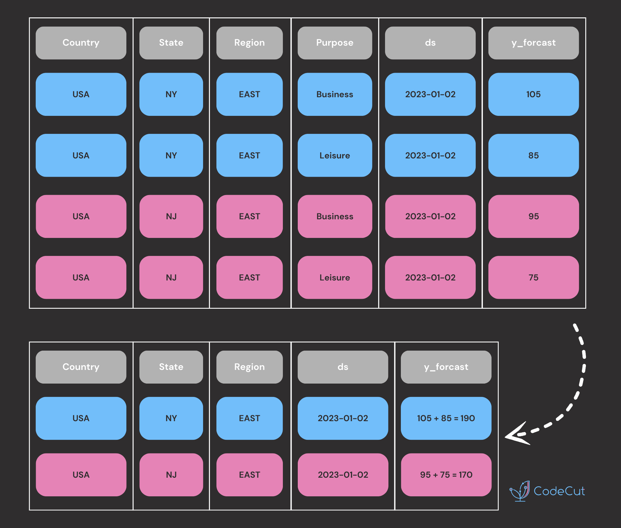
First, forecasts are created at the most detailed level: Country, State, Region, Purpose. For example, the forecast for the next date might look like this:
| Country | State | Region | Purpose | ds | y_forecast |
|---|---|---|---|---|---|
| USA | NY | East | Business | 2023-01-02 | 105 |
| USA | NY | East | Leisure | 2023-01-02 | 85 |
| USA | NJ | East | Business | 2023-01-02 | 95 |
| USA | NJ | East | Leisure | 2023-01-02 | 75 |
| USA | CA | West | Business | 2023-01-02 | 125 |
| USA | CA | West | Leisure | 2023-01-02 | 115 |
| USA | NV | West | Business | 2023-01-02 | 65 |
| USA | NV | West | Leisure | 2023-01-02 | 55 |
Country, State, Purpose
Sum the forecasts for each Country, State, Purpose combination.
| Country | State | Purpose | ds | y_forecast |
|---|---|---|---|---|
| USA | NY | Business | 2023-01-02 | 105 |
| USA | NY | Leisure | 2023-01-02 | 85 |
| USA | NJ | Business | 2023-01-02 | 95 |
| USA | NJ | Leisure | 2023-01-02 | 75 |
| USA | CA | Business | 2023-01-02 | 125 |
| USA | CA | Leisure | 2023-01-02 | 115 |
| USA | NV | Business | 2023-01-02 | 65 |
| USA | NV | Leisure | 2023-01-02 | 55 |
Country, State, Region
Sum the forecasts for each Country, State, Region combination.
| Country | State | Region | ds | y_forecast |
|---|---|---|---|---|
| USA | NY | East | 2023-01-02 | 190 |
| USA | NJ | East | 2023-01-02 | 170 |
| USA | CA | West | 2023-01-02 | 240 |
| USA | NV | West | 2023-01-02 | 120 |
Country, Purpose
Sum the forecasts for each Country, Purpose combination.
| Country | Purpose | ds | y_forecast |
|---|---|---|---|
| USA | Business | 2023-01-02 | 390 |
| USA | Leisure | 2023-01-02 | 330 |
Country
Sum the forecasts for the entire Country.
| Country | ds | y_forecast |
|---|---|---|
| USA | 2023-01-02 | 720 |
Conclusion
Hierarchical forecasting solves one of the most common pain points in multi-level time series work: forecasts that don’t add up across a hierarchy. Instead of manually reconciling regional totals with national forecasts after the fact, HierarchicalForecast from Nixtla builds consistency into the forecasting step itself. This matters for any team that reports at multiple granularities — sales by country and by region, inventory by warehouse and by SKU, demand by category and by product. Reconciled forecasts mean every stakeholder is working from the same numbers, and decisions made at the executive level don’t contradict what operations teams are planning on the ground.
If you’re already using statsmodels, Prophet, or scikit-learn for forecasting but finding that your aggregates don’t match, HierarchicalForecast is designed to plug in alongside them. You get a principled reconciliation layer (bottom-up, top-down, or optimal combination methods) without having to rewrite your base models.
Read Next
Processing large time series data? Read our deep dive: pandas vs Polars vs DuckDB: A Data Scientist’s Guide. Find the fastest tool for your data workloads.


