Motivation

Time series forecasting often requires incorporating external factors that can influence the target variable. However, handling these external factors (exogenous features) can be complex, especially when some features remain constant while others change over time.

# Example without proper handling of exogenous features
import pandas as pd

# Sales data with product info and prices
data = pd.DataFrame({
    'date': ['2024-01-01', '2024-01-02', '2024-01-03'],
    'product_id': [1, 1, 1],
    'category': ['electronics', 'electronics', 'electronics'],
    'price': [99.99, 89.99, 94.99],
    'sales': [150, 200, 175]
})

# Difficult to handle static (category) vs dynamic (price) features
# Risk of data leakage or incorrect feature engineering

This code shows the challenge of handling both static features (product category) and dynamic features (price) in time series forecasting. Without proper handling, you might incorrectly use future information or miss important patterns in the data.

Understanding Features in Time Series

Before diving into MLForecast, let’s understand two important concepts:

1. Static features: These are features that don’t change over time (like product category or location)
2. Dynamic features (exogenous): These are features that change over time (like price or weather)

Introduction to MLForecast

MLForecast is a Python library that simplifies time series forecasting with machine learning models while properly handling both static and dynamic features. It can be installed using:

pip install mlforecast

As covered in the past article about MLForecast’s workflow, it provides an integrated approach to time series forecasting. In this post, we will focus on its exogenous features capabilities.

Working with Exogenous Features

MLForecast makes it easy to handle both static and dynamic features in your forecasting models. Here’s how:

First, let’s prepare our data with both types of features:

import lightgbm as lgb
from mlforecast import MLForecast
from mlforecast.utils import generate_daily_series, generate_prices_for_series

# Generate sample data
series = generate_daily_series(100, equal_ends=True, n_static_features=2)
series = series.rename(columns={'static_1': 'product_id'})

# Generate price catalog (dynamic feature)
prices_catalog = generate_prices_for_series(series)

# Merge static and dynamic features
series_with_prices = series.merge(prices_catalog, how='left')
print(series_with_prices.head(10))

Output:

  unique_id         ds           y store_id product_id     price
0     id_00 2000-10-05   39.811983       79         45  0.548814
1     id_00 2000-10-06  103.274013       79         45  0.715189
2     id_00 2000-10-07  176.574744       79         45  0.602763
3     id_00 2000-10-08  258.987900       79         45  0.544883
4     id_00 2000-10-09  344.940404       79         45  0.423655
5     id_00 2000-10-10  413.520305       79         45  0.645894
6     id_00 2000-10-11  506.990093       79         45  0.437587
7     id_00 2000-10-12   12.688070       79         45  0.891773
8     id_00 2000-10-13  111.133819       79         45  0.963663
9     id_00 2000-10-14  197.982842       79         45  0.383442

Now, let’s create and train our model:

# Create MLForecast model
fcst = MLForecast(
    models=lgb.LGBMRegressor(random_state=0),
    freq="D",
    lags=[7],  # Use 7-day lag
    date_features=["dayofweek"],  # Add day of week as feature
)

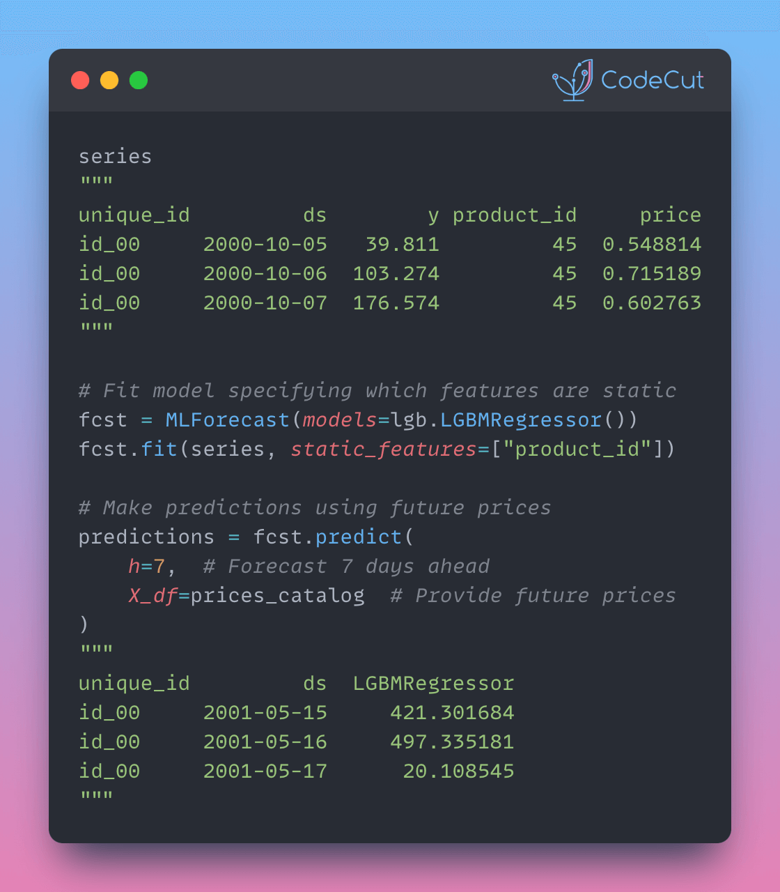
# Fit model specifying which features are static
fcst.fit(
    series_with_prices,
    static_features=["store_id", "product_id"],  # Specify static features
)

# Check which features are used for training
print("\nFeatures used for training:")
print(fcst.ts.features_order_)

Output:

Features used for training:
['store_id', 'product_id', 'price', 'lag7', 'dayofweek']

Generate predictions:

# Make predictions using future prices
predictions = fcst.predict(
    h=7,  # Forecast 7 days ahead
    X_df=prices_catalog  # Provide future prices
)
predictions.head(10)

Output:

  unique_id         ds  LGBMRegressor
0     id_00 2001-05-15     421.301684
1     id_00 2001-05-16     497.335181
2     id_00 2001-05-17      20.108545
3     id_00 2001-05-18     101.930145
4     id_00 2001-05-19     184.264253
5     id_00 2001-05-20     260.803990
6     id_00 2001-05-21     343.501305
7     id_01 2001-05-15     118.299009
8     id_01 2001-05-16     148.793503
9     id_01 2001-05-17     184.066779

The output shows forecasted values that take into account both static features (product information) and dynamic features (prices).

MLForecast vs Traditional Approaches

Traditional approaches often require separate handling of static and dynamic features, leading to complex preprocessing pipelines. MLForecast simplifies this by:

1. Automatically managing feature types
2. Preventing data leakage
3. Providing an integrated workflow

Conclusion

MLForecast’s handling of exogenous features significantly simplifies time series forecasting by providing a clean interface for both static and dynamic features. This makes it easier to incorporate external information into your forecasts while maintaining proper time series practices.

Link to MLForecast