Table of Contents

• Introduction
• From Pandas UDFs to Arrow UDFs: Next-Gen Performance
• Native Data Visualization (PySpark 4.0+)
• Schema-Free JSON Handling with Variant Type (PySpark 4.0+)
• Dynamic Schema Generation with UDTF analyze() (PySpark 4.0+)
• Conclusion

Introduction

PySpark 4.0 introduces transformative improvements that enhance performance, streamline workflows, and enable flexible data transformations in distributed processing.

This release delivers four key enhancements:

• Arrow-optimized UDFs accelerate custom transformations by operating directly on Arrow data structures, eliminating the serialization overhead of Pandas UDFs.
• Native Plotly visualization enables direct DataFrame plotting without conversion, streamlining exploratory data analysis and reducing memory overhead.
• Variant type for JSON enables schema-free JSON querying with JSONPath syntax, eliminating verbose StructType definitions for nested data.
• Dynamic schema UDTFs adapt output columns to match input data at runtime, enabling flexible pivot tables and aggregations where column structure depends on data values.

For comprehensive coverage of core PySpark SQL functionality, see the Complete Guide to PySpark SQL.

From Pandas UDFs to Arrow UDFs: Next-Gen Performance

The pandas_udf function requires converting Arrow data to Pandas format and back again for each operation. This serialization cost becomes significant when processing large datasets.

PySpark 3.5+ introduces Arrow-optimized UDFs via the useArrow=True parameter, which operates directly on Arrow data structures, avoiding the Pandas conversion entirely and improving performance.

Let’s compare the performance with a weighted sum calculation across multiple columns on 100,000 rows:

import pandas as pd
import pyarrow.compute as pc
from pyspark.sql import SparkSession
from pyspark.sql.functions import pandas_udf, udf
from pyspark.sql.types import DoubleType


spark = SparkSession.builder.appName("UDFComparison").getOrCreate()

# Create test data with multiple numeric columns
data = [(float(i), float(i*2), float(i*3)) for i in range(100000)]
df = spark.createDataFrame(data, ["val1", "val2", "val3"])

Create a timing decorator to measure the execution time of the functions:

import time
from functools import wraps


# Timing decorator
def timer(func):
    @wraps(func)
    def wrapper(*args, **kwargs):
        start = time.time()
        result = func(*args, **kwargs)
        elapsed = time.time() - start
        print(f"{func.__name__}: {elapsed:.2f}s")
        wrapper.elapsed_time = elapsed
        return result

    return wrapper

Use the timing decorator to measure the execution time of the pandas_udf function:

@pandas_udf(DoubleType())
def weighted_sum_pandas(v1: pd.Series, v2: pd.Series, v3: pd.Series) -> pd.Series:
    return v1 * 0.5 + v2 * 0.3 + v3 * 0.2

@timer
def run_pandas_udf():
    result = df.select(
        weighted_sum_pandas(df.val1, df.val2, df.val3).alias("weighted")
    )
    result.count()  # Trigger computation
    return result

result_pandas = run_pandas_udf()
pandas_time = run_pandas_udf.elapsed_time

run_pandas_udf: 1.33s

Use the timing decorator to measure the execution time of the Arrow-optimized UDF using useArrow:

from pyspark.sql.functions import udf
from pyspark.sql.types import DoubleType

@udf(DoubleType(), useArrow=True)
def weighted_sum_arrow(v1, v2, v3):
    term1 = pc.multiply(v1, 0.5)
    term2 = pc.multiply(v2, 0.3)
    term3 = pc.multiply(v3, 0.2)
    return pc.add(pc.add(term1, term2), term3)

@timer
def run_arrow_udf():
    result = df.select(
        weighted_sum_arrow(df.val1, df.val2, df.val3).alias("weighted")
    )
    result.count()  # Trigger computation
    return result

result_arrow = run_arrow_udf()
arrow_time = run_arrow_udf.elapsed_time

run_arrow_udf: 0.43s

Measure the speedup:

speedup = pandas_time / arrow_time
print(f"Speedup: {speedup:.2f}x faster")

Speedup: 3.06x faster

The output shows that the Arrow-optimized version is 3.06x faster than the pandas_udf version!

The performance gain comes from avoiding serialization. Arrow-optimized UDFs use PyArrow compute functions like pc.multiply() and pc.add() directly on Arrow data, while pandas_udf must convert each column to Pandas and back.

Trade-off: The 3.06x performance improvement comes at the cost of using PyArrow’s less familiar compute API instead of Pandas operations. However, this becomes increasingly valuable as dataset size and column count grow.

Native Data Visualization (PySpark 4.0+)

Visualizing PySpark DataFrames traditionally requires converting to Pandas first, then using external libraries like matplotlib or plotly. This adds memory overhead and extra processing steps.

PySpark 4.0 introduces a native plotting API powered by Plotly, enabling direct visualization from PySpark DataFrames without any conversion.

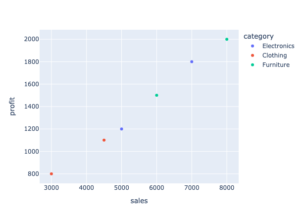
Let’s visualize sales data across product categories:

from pyspark.sql import SparkSession

spark = SparkSession.builder.appName("Visualization").getOrCreate()

# Create sample sales data
sales_data = [
    ("Electronics", 5000, 1200),
    ("Electronics", 7000, 1800),
    ("Clothing", 3000, 800),
    ("Clothing", 4500, 1100),
    ("Furniture", 6000, 1500),
    ("Furniture", 8000, 2000),
]

sales_df = spark.createDataFrame(sales_data, ["category", "sales", "profit"])
sales_df.show()

+-----------+-----+------+
|   category|sales|profit|
+-----------+-----+------+
|Electronics| 5000|  1200|
|Electronics| 7000|  1800|
|   Clothing| 3000|   800|
|   Clothing| 4500|  1100|
|  Furniture| 6000|  1500|
|  Furniture| 8000|  2000|
+-----------+-----+------+

Create a scatter plot directly from the PySpark DataFrame using the .plot() method:

# Direct plotting without conversion
sales_df.plot(kind="scatter", x="sales", y="profit", color="category")

You can also use shorthand methods such as plot.scatter() and plot.bar() for specific chart types:

# Scatter plot with shorthand
sales_df.plot.scatter(x="sales", y="profit", color="category")

# Bar chart by category
category_totals = sales_df.groupBy("category").agg({"sales": "sum"}).withColumnRenamed("sum(sales)", "total_sales")
category_totals.plot.bar(x="category", y="total_sales")

The native plotting API supports 8 chart types:

• scatter: Scatter plots with color grouping
• bar: Bar charts for categorical comparisons
• line: Line plots for time series
• area: Area charts for cumulative values
• pie: Pie charts for proportions
• box: Box plots for distributions
• histogram: Histograms for frequency analysis
• kde/density: Density plots for probability distributions

By default, PySpark visualizes up to 1,000 rows. For larger datasets, configure the limit:

# Increase visualization row limit
spark.conf.set("spark.sql.pyspark.plotting.max_rows", 5000)

Schema-Free JSON Handling with Variant Type (PySpark 4.0+)

Extracting nested JSON in PySpark requires defining StructType schemas that mirror your data structure. This creates verbose code that breaks whenever your JSON changes.

Let’s extract data from a 3-level nested JSON structure using the traditional approach:

from pyspark.sql import SparkSession
from pyspark.sql.types import StructType, StructField, StringType

spark = SparkSession.builder.appName("json_schema").getOrCreate()

# 3 levels of nested StructType - verbose and hard to maintain
schema = StructType([
    StructField("user", StructType([
        StructField("name", StringType()),
        StructField("profile", StructType([
            StructField("settings", StructType([
                StructField("theme", StringType())
            ]))
        ]))
    ]))
])

json_data = [
    '{"user": {"name": "Alice", "profile": {"settings": {"theme": "dark"}}}}',
    '{"user": {"name": "Bob", "profile": {"settings": {"theme": "light"}}}}'
]

rdd = spark.sparkContext.parallelize(json_data)
df = spark.read.schema(schema).json(rdd)
df.select("user.name", "user.profile.settings.theme").show()

+-----+-----+
| name|theme|
+-----+-----+
|Alice| dark|
|  Bob|light|
+-----+-----+

PySpark 4.0 introduces the Variant type, which lets you skip schema definitions entirely. To work with the Variant type:

• Use parse_json() to load JSON data
• Use variant_get() to extract fields with JSONPath syntax

from pyspark.sql import SparkSession
from pyspark.sql.functions import parse_json, variant_get

spark = SparkSession.builder.appName("json_variant").getOrCreate()

json_data = [
    ('{"user": {"name": "Alice", "profile": {"settings": {"theme": "dark"}}}}',),
    ('{"user": {"name": "Bob", "profile": {"settings": {"theme": "light"}}}}',)
]

df = spark.createDataFrame(json_data, ["json_str"])
df_variant = df.select(parse_json("json_str").alias("data"))

# No schema needed - just use JSONPath
result = df_variant.select(
    variant_get("data", "$.user.name", "string").alias("name"),
    variant_get("data", "$.user.profile.settings.theme", "string").alias("theme")
)
result.show()

+-----+-----+
| name|theme|
+-----+-----+
|Alice| dark|
|  Bob|light|
+-----+-----+

The Variant type provides several advantages:

• No upfront schema definition: Handle any JSON structure without verbose StructType definitions
• JSONPath syntax: Access nested paths using $.path.to.field notation regardless of depth
• Schema flexibility: JSON structure changes don’t break your code
• Type safety: variant_get() lets you specify the expected type when extracting fields

Dynamic Schema Generation with UDTF analyze() (PySpark 4.0+)

Python UDTFs (User-Defined Table Functions) generate multiple rows from a single input row, but they come with a critical limitation: you must define the output schema upfront. When your output columns depend on the input data itself (like creating pivot tables or dynamic aggregations where column names come from data values), this rigid schema requirement becomes a problem.

For example, a word-counting UDTF requires you to specify all output columns upfront, even though the words themselves are unknown until runtime.

from pyspark.sql.functions import udtf, lit
from pyspark.sql.types import StructType, StructField, IntegerType

# Schema must be defined upfront with fixed column names
@udtf(returnType=StructType([
    StructField("hello", IntegerType()),
    StructField("world", IntegerType()),
    StructField("spark", IntegerType())
]))
class StaticWordCountUDTF:
    def eval(self, text: str):
        words = text.split(" ")
        yield tuple(words.count(word) for word in ["hello", "world", "spark"])

# Only works for exactly these three words
result = StaticWordCountUDTF(lit("hello world hello spark"))
result.show()

+-----+-----+-----+
|hello|world|spark|
+-----+-----+-----+
|    2|    1|    1|
+-----+-----+-----+

If the input text contains a different set of words, the output won’t contain the count of the new words.

result = StaticWordCountUDTF(lit("hi world hello spark"))
result.show()

+-----+-----+-----+
|hello|world|spark|
+-----+-----+-----+
|    1|    1|    1|
+-----+-----+-----+

PySpark 4.0 introduces the analyze() method for UDTFs, enabling dynamic schema determination based on input data. Instead of hardcoding your output schema, analyze() inspects the input and generates the appropriate columns at runtime.

from pyspark.sql.functions import udtf, lit
from pyspark.sql.types import StructType, IntegerType
from pyspark.sql.udtf import AnalyzeArgument, AnalyzeResult

@udtf
class DynamicWordCountUDTF:
    @staticmethod
    def analyze(text: AnalyzeArgument) -> AnalyzeResult:
        """Dynamically create schema based on input text"""
        schema = StructType()
        # Create one column per unique word in the input
        for word in sorted(set(text.value.split(" "))):
            schema = schema.add(word, IntegerType())
        return AnalyzeResult(schema=schema)

    def eval(self, text: str):
        """Generate counts for each word"""
        words = text.split(" ")
        # Use same logic as analyze() to determine column order
        unique_words = sorted(set(words))
        yield tuple(words.count(word) for word in unique_words)

# Schema adapts to any input text
result = DynamicWordCountUDTF(lit("hello world hello spark"))
result.show()

+-----+-----+-----+
|hello|spark|world|
+-----+-----+-----+
|    2|    1|    1|
+-----+-----+-----+

Now try with completely different words:

# Different words - schema adapts automatically
result2 = DynamicWordCountUDTF(lit("python data science"))
result2.show()

+----+------+-------+
|data|python|science|
+----+------+-------+
|   1|     1|      1|
+----+------+-------+

The columns change from hello, spark, world to data, python, science without any code modifications.

Conclusion

PySpark 4.0 makes distributed computing faster and easier to use. Arrow-optimized UDFs speed up custom transformations, the Variant type simplifies JSON handling, native visualization removes conversion steps, and dynamic UDTFs handle flexible data structures.

These improvements address real bottlenecks without requiring major code changes, making PySpark more practical for everyday data engineering tasks.

📚 Want to go deeper? Learning new techniques is the easy part. Knowing how to structure, test, and deploy them is what separates side projects from real work. My book shows you how to build data science projects that actually make it to production. Get the book →