Table of Contents

• Introduction
• Tool Selection Guide
• Setting Up the Environment
• IPython.display.Latex: Built-in LaTeX Rendering
• handcalcs: Step-by-Step Calculations
• latexify-py: Automated Function Conversion
• SymPy: Symbolic Mathematics
• Final Thoughts

Introduction

Imagine you are a financial analyst, who is building financial models in Python and need to present them to non-technical executives. Since they are not familiar with Python, you need to show them the mathematical foundations behind your algorithms, not just code blocks. How can you do that?

The best way to present mathematical models is to use LaTeX. It is a powerful tool for writing mathematical notation and equations. It is widely used in academic papers, research papers, and technical reports.

However, writing LaTeX by hand is not easy, especially for complex equations. In this article, you will learn how to convert Python code to LaTeX in Jupyter notebooks using four powerful tools: IPython.display.Latex, handcalcs, latexify-py, and SymPy.

💻 Get the Code: The complete source code and Jupyter notebook for this tutorial are available on GitHub. Clone it to follow along!

Key Takeaways

Here’s what you’ll learn:

• Transform Python calculations into professional LaTeX equations using four specialized tools
• Generate step-by-step mathematical documentation automatically with handcalcs magic commands
• Convert Python functions to clean LaTeX notation instantly using latexify-py decorators
• Perform symbolic mathematics including equation solving and algebraic manipulation with SymPy

Setting Up the Environment

Install the required packages using pip or uv.

# Using pip
pip install handcalcs latexify-py sympy

# Using uv (recommended)
uv add handcalcs latexify-py sympy

📚 For production-ready notebook workflows and development best practices, check out Production-Ready Data Science.

IPython.display.Latex: Built-in LaTeX Rendering

The simplest approach uses Jupyter’s built-in IPython.display.Latex rendering. It is ideal when you want precise control over mathematical notation.

Let’s create a professional-looking compound interest calculation.

Start with defining the variables, where P is the principal amount, r is the annual interest rate, and t is the number of years.

P = 10000 # principal amount
r = 0.08 # annual interest rate
t = 5 # number of years

Now we are ready to display the calculation in LaTeX. To make the calculation easier to follow, we will break it down into three parts:

• Display the formula
• Substitute the variables into the formula
• Display the result

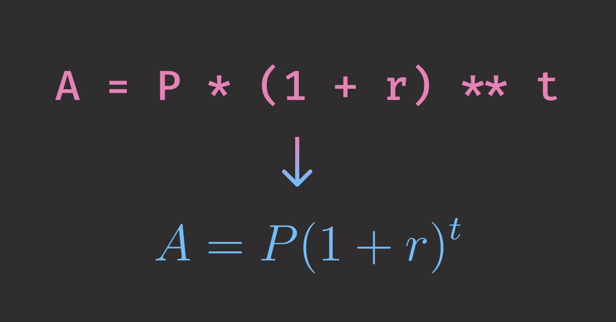
# Calculate result
A = P * (1 + r) ** t

# Display the calculation with LaTeX
display(Latex(r"$A = P(1 + r)^t$"))
display(Latex(f"$A = {P:,}(1 + {r})^{{{t}}}$"))
display(Latex(f"$A = {A:,.2f}$"))

This shows step-by-step substitutions, but writing LaTeX for each step is manual and slow.

Wouldn’t it be nice if we could have steps and substitutions and latex code automatically generated when writing Python code? That is where handcalcs comes in.

handcalcs: Step-by-Step Calculations

handcalcs automatically converts Python calculations into step-by-step mathematical documentation. It’s perfect for technical reports and educational content.

Jupyter Magic Command

To use handcals in Jupyter, we need to load the extension first.

import handcalcs.render
from handcalcs import handcalc

# Enable handcalcs in Jupyter
%load_ext handcalcs.render

Now we can use the %%render magic command to render the calculation.

%%render
# Step-by-step substitutions for compound interest
A = P * (1 + r)**t

This renders as a complete step-by-step calculation showing all substitutions and intermediate results. All without writing a single line of LaTeX code!

Function Decorator

Use the function decorator to render calculations. Set jupyter_display=True to show the LaTeX in Jupyter.

from handcalcs import handcalc

@handcalc(jupyter_display=True)
def calculate_compound_interest(P, r, t):
    A = P * (1 + r)**t
    return A

# Calling the function renders the calculation with substitutions
result = calculate_compound_interest(10000, 0.08, 5)

The result is a simple number that can be used for further calculations.

result
print(f"Result: {result:,.2f}")

Output:

Result: 14,693.28

latexify-py: Automated Function Conversion

Unlike handcalcs, which renders step-by-step numeric substitutions, latexify-py focuses on function-level documentation without the intermediate arithmetic. It’s ideal when you want a clean, reusable formula and don’t need to show the intermediate steps.

import latexify


# Simple function conversion
@latexify.function
def A(P, r, t):
    return P * (1 + r) ** t

A

The latexify-py function can be used like a normal Python function to compute the result.

result = A(10000, 0.08, 5)
print(f"Result: {result:,.2f}")

Output:

Result: 14,693.28

SymPy: Symbolic Mathematics

handcalcs and latexify-py excel at rendering clear results from concrete values, but they are not good at symbolic tasks like solving variables, computing derivatives or integrals. For these tasks, use SymPy.

To create a symbolic equation, start with defining the variables and the equation.

from sympy import symbols, Eq, solve

# Define the variables
A, P, r, t = symbols("A P r t", positive=True)

# Define the equation
eq = Eq(A, P * (1 + r) ** t)
eq

After setting up the equation, we are ready to perform symbolic calculations.

Substitute Variables

Let’s compute A (amount) from given P (principal), r (interest rate), and t (time) by solving for A and substituting values.

# Solve for A
A_expr = solve(eq, A)[0]

# Substitute the values
A_result = A_expr.subs({P: 10000, r: 0.08, t: 5})
A_result

Solve for a Variable

Let’s solve the equation for t to answer the question: “How many years will it take for the investment to reach A (amount) given P (principal) and r (interest rate)?”

t_sol = solve(eq, t)[0]
t_sol

The result is the formula to solve for t.

Now we can substitute the variables into the equation to answer a more specific question: “How many years will it take for the investment to reach $5,000 given a principal of $1,000 and an annual interest rate of 8%?”

t_result = t_sol.subs({P: 1000, r: 0.08, A: 5000}).evalf(2)
t_result

The result shows that it will take approximately 21 years for the investment to reach $5,000.

Expand and Factor an Expression

We can also use SymPy to expand and factor an expression.

Assume t = 2. With an annual rate r and two compounding periods, the expression becomes:

compound_expr = P * (1 + r) ** 2
compound_expr

Let’s expand the expression using the expand function.

from sympy import expand

expanded_expr = expand(compound_expr)
expanded_expr

We can then turn the expression back into a product of factors using the factor function.

from sympy import factor

factored_expr = factor(expanded_expr)
factored_expr

Summary

Converting Python code to LaTeX in Jupyter notebooks transforms your technical documentation from code-heavy to mathematically elegant. Here’s when to use each tool:

• Use IPython.display.Latex when: You need precise control over mathematical notation
• Use handcalcs when: You want step-by-step calculation documentation
• Use latexify-py when: You want automatic function-to-LaTeX conversion
• Use SymPy when: You want to solve equations, compute derivatives and integrals

Related Tutorials

• Broader Visualization: Top 6 Python Libraries for Visualization: Which One to Use? for comprehensive visualization options beyond mathematical notation
• Advanced Mathematical Operations: 5 Essential Itertools for Data Science for complex mathematical workflows and performance optimization