Traditionally, data scientists need to manually code and test multiple models, which is time-consuming and labor-intensive.

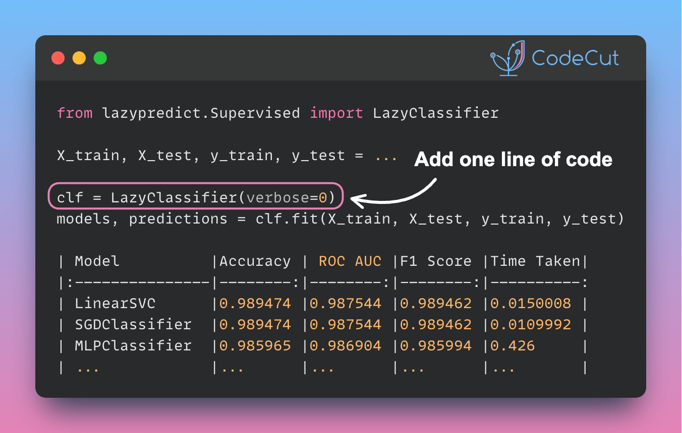
Lazy Predict enables rapid prototyping and comparison of multiple basic models without extensive manual coding or parameter tuning.

This helps data scientists identify promising approaches and iterate on them more quickly.

Here’s a practical example using the breast cancer dataset:

from lazypredict.Supervised import LazyClassifier
from sklearn.datasets import load_breast_cancer
from sklearn.model_selection import train_test_split

data = load_breast_cancer()
X = data.data
y= data.target

X_train, X_test, y_train, y_test = train_test_split(X, y,test_size=.5,random_state =123)

clf = LazyClassifier(verbose=0, ignore_warnings=True, custom_metric=None)
models, predictions = clf.fit(X_train, X_test, y_train, y_test)

print(models)

This code snippet generates a comprehensive comparison of various classification models, evaluating them on metrics such as accuracy, balanced accuracy, ROC AUC, and F1 score. The output is a table ranking models by performance, allowing quick identification of the most promising algorithms for the given dataset.

| Model                          |   Accuracy |   Balanced Accuracy |   ROC AUC |   F1 Score |   Time Taken |
|:-------------------------------|-----------:|--------------------:|----------:|-----------:|-------------:|
| LinearSVC                      |   0.989474 |            0.987544 |  0.987544 |   0.989462 |    0.0150008 |
| SGDClassifier                  |   0.989474 |            0.987544 |  0.987544 |   0.989462 |    0.0109992 |
| MLPClassifier                  |   0.985965 |            0.986904 |  0.986904 |   0.985994 |    0.426     |
| Perceptron                     |   0.985965 |            0.984797 |  0.984797 |   0.985965 |    0.0120046 |
| LogisticRegression             |   0.985965 |            0.98269  |  0.98269  |   0.985934 |    0.0200036 |
| LogisticRegressionCV           |   0.985965 |            0.98269  |  0.98269  |   0.985934 |    0.262997  |
| SVC                            |   0.982456 |            0.979942 |  0.979942 |   0.982437 |    0.0140011 |
| CalibratedClassifierCV         |   0.982456 |            0.975728 |  0.975728 |   0.982357 |    0.0350015 |
| PassiveAggressiveClassifier    |   0.975439 |            0.974448 |  0.974448 |   0.975464 |    0.0130005 |
| LabelPropagation               |   0.975439 |            0.974448 |  0.974448 |   0.975464 |    0.0429988 |
| LabelSpreading                 |   0.975439 |            0.974448 |  0.974448 |   0.975464 |    0.0310006 |
| RandomForestClassifier         |   0.97193  |            0.969594 |  0.969594 |   0.97193  |    0.033     |
| GradientBoostingClassifier     |   0.97193  |            0.967486 |  0.967486 |   0.971869 |    0.166998  |
| QuadraticDiscriminantAnalysis  |   0.964912 |            0.966206 |  0.966206 |   0.965052 |    0.0119994 |
| HistGradientBoostingClassifier |   0.968421 |            0.964739 |  0.964739 |   0.968387 |    0.682003  |
| RidgeClassifierCV              |   0.97193  |            0.963272 |  0.963272 |   0.971736 |    0.0130029 |
| RidgeClassifier                |   0.968421 |            0.960525 |  0.960525 |   0.968242 |    0.0119977 |
| AdaBoostClassifier             |   0.961404 |            0.959245 |  0.959245 |   0.961444 |    0.204998  |
| ExtraTreesClassifier           |   0.961404 |            0.957138 |  0.957138 |   0.961362 |    0.0270066 |
| KNeighborsClassifier           |   0.961404 |            0.95503  |  0.95503  |   0.961276 |    0.0560005 |
| BaggingClassifier              |   0.947368 |            0.954577 |  0.954577 |   0.947882 |    0.0559971 |
| BernoulliNB                    |   0.950877 |            0.951003 |  0.951003 |   0.951072 |    0.0169988 |
| LinearDiscriminantAnalysis     |   0.961404 |            0.950816 |  0.950816 |   0.961089 |    0.0199995 |
| GaussianNB                     |   0.954386 |            0.949536 |  0.949536 |   0.954337 |    0.0139935 |
| NuSVC                          |   0.954386 |            0.943215 |  0.943215 |   0.954014 |    0.019989  |
| DecisionTreeClassifier         |   0.936842 |            0.933693 |  0.933693 |   0.936971 |    0.0170023 |
| NearestCentroid                |   0.947368 |            0.933506 |  0.933506 |   0.946801 |    0.0160074 |
| ExtraTreeClassifier            |   0.922807 |            0.912168 |  0.912168 |   0.922462 |    0.0109999 |
| CheckingClassifier             |   0.361404 |            0.5      |  0.5      |   0.191879 |    0.0170043 |
| DummyClassifier                |   0.512281 |            0.489598 |  0.489598 |   0.518924 |    0.0119965 |

The top-performing models in this case are:

1. LinearSVC (Accuracy: 0.989, ROC AUC: 0.988)
2. SGDClassifier (Accuracy: 0.989, ROC AUC: 0.988)
3. MLPClassifier (Accuracy: 0.986, ROC AUC: 0.987)

Link to Lazy Predict.