
Time series cross-validation evaluates a model’s predictive performance by training on past data and testing on subsequent time periods using a sliding window approach.
MLForecast offers an efficient and easy-to-use implementation of this technique.
To see how to implement time series cross-validation with MLForecast, let’s start reading a subset of the M4 Competition hourly dataset.
import pandas as pd
from utilsforecast.plotting import plot_series

Y_df = pd.read_csv("https://datasets-nixtla.s3.amazonaws.com/m4-hourly.csv").query(
    "unique_id == 'H1'"
)
Y_df
unique_id ds y
0 H1 1 605.0
1 H1 2 586.0
2 H1 3 586.0
3 H1 4 559.0
4 H1 5 511.0
.. ... ... ...
743 H1 744 785.0
744 H1 745 756.0
745 H1 746 719.0
746 H1 747 703.0
747 H1 748 659.0
[748 rows x 3 columns]Plot the time series:
fig = plot_series(Y_df, plot_random=False, max_insample_length=24 * 14)
fig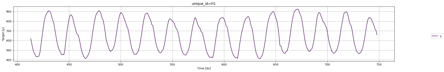
Instantiate a new MLForecast object:
from mlforecast import MLForecast
from mlforecast.target_transforms import Differences
from sklearn.linear_model import LinearRegression


mlf = MLForecast(
    models=[LinearRegression()],
    freq=1,
    target_transforms=[Differences([24])],
    lags=range(1, 25),
)
Once the MLForecast object has been instantiated, we can use the cross_validation method.
For this particular example, we’ll use 3 windows of 24 hours.
# use 3 windows of 24 hours
cross_validation_df = mlf.cross_validation(
    df=Y_df,
    h=24,
    n_windows=3,
)
cross_validation_df.head()
unique_id ds cutoff y LinearRegression
0 H1 677 676 691.0 676.726797
1 H1 678 676 618.0 559.559522
2 H1 679 676 563.0 549.167938
3 H1 680 676 529.0 505.930997
4 H1 681 676 504.0 481.981893
We’ll now plot the forecast for each cutoff period.
import matplotlib.pyplot as plt


def plot_cv(df, df_cv, last_n=24 * 14):
    cutoffs = df_cv["cutoff"].unique()
    fig, ax = plt.subplots(
        nrows=len(cutoffs), ncols=1, figsize=(14, 6), gridspec_kw=dict(hspace=0.8)
    )
    for cutoff, axi in zip(cutoffs, ax.flat):
        df.tail(last_n).set_index("ds").plot(ax=axi, y="y")
        df_cv.query("cutoff == @cutoff").set_index("ds").plot(
            ax=axi,
            y="LinearRegression",
            title=f"{cutoff=}",
        )


plot_cv(Y_df, cross_validation_df)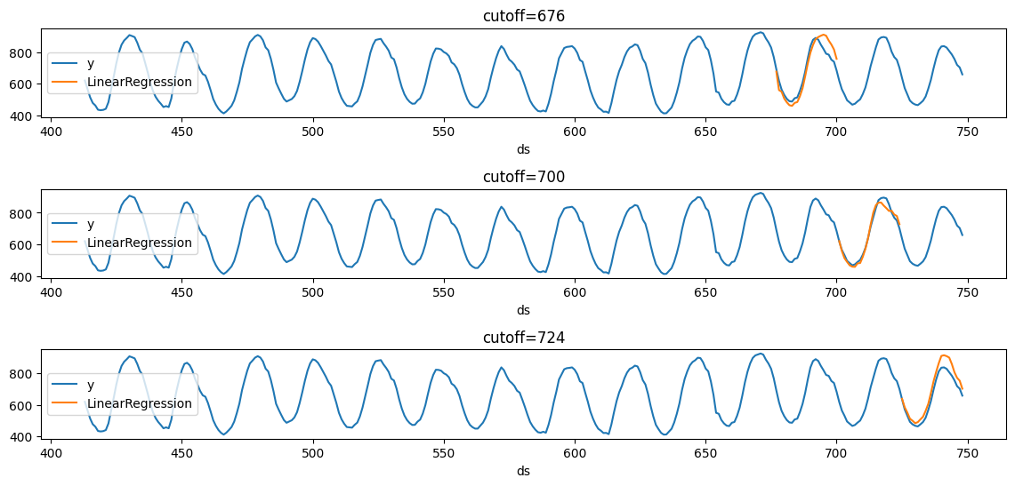
Notice that in each cutoff period, we generated a forecast for the next 24 hours using only the data y before said period.