Generic selectors
Exact matches only
Search in title
Search in content
Post Type Selectors
Filter by Categories
About Article
Analyze Data
Archive
Best Practices
Better Outputs
Blog
Code Optimization
Code Quality
Command Line
Daily tips
Dashboard
Data Analysis & Manipulation
Data Engineer
Data Visualization
DataFrame
Delta Lake
DevOps
DuckDB
Environment Management
Feature Engineer
Git
Jupyter Notebook
LLM
LLM Tools
Machine Learning
Machine Learning & AI
Machine Learning Tools
Manage Data
MLOps
Natural Language Processing
NumPy
Pandas
Polars
PySpark
Python Helpers
Python Tips
Python Utilities
Scrape Data
SQL
Testing
Time Series
Tools
Visualization
Visualization & Reporting
Workflow & Automation
Workflow Automation

Python Tips

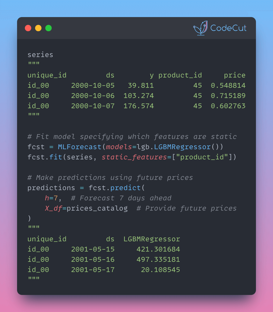
MLForecast: Automate External Feature Handling

Motivation

Time series forecasting often requires incorporating external factors that can influence the target variable. However, handling these external factors (exogenous features) can be complex, especially when some features remain constant while others change over time.

# Example without proper handling of exogenous features
import pandas as pd

# Sales data with product info and prices
data = pd.DataFrame({
'date': ['2024-01-01', '2024-01-02', '2024-01-03'],
'product_id': [1, 1, 1],
'category': ['electronics', 'electronics', 'electronics'],
'price': [99.99, 89.99, 94.99],
'sales': [150, 200, 175]
})

# Difficult to handle static (category) vs dynamic (price) features
# Risk of data leakage or incorrect feature engineering

This code shows the challenge of handling both static features (product category) and dynamic features (price) in time series forecasting. Without proper handling, you might incorrectly use future information or miss important patterns in the data.

Understanding Features in Time Series

Before diving into MLForecast, let’s understand two important concepts:

Static features: These are features that don’t change over time (like product category or location)

Dynamic features (exogenous): These are features that change over time (like price or weather)

Introduction to MLForecast

MLForecast is a Python library that simplifies time series forecasting with machine learning models while properly handling both static and dynamic features. It can be installed using:

pip install mlforecast

As covered in the past article about MLForecast’s workflow, it provides an integrated approach to time series forecasting. In this post, we will focus on its exogenous features capabilities.

Working with Exogenous Features

MLForecast makes it easy to handle both static and dynamic features in your forecasting models. Here’s how:

First, let’s prepare our data with both types of features:

import lightgbm as lgb
from mlforecast import MLForecast
from mlforecast.utils import generate_daily_series, generate_prices_for_series

# Generate sample data
series = generate_daily_series(100, equal_ends=True, n_static_features=2)
series = series.rename(columns={"static_0": "store_id", "static_1": "product_id"})

# Generate price catalog (dynamic feature)
prices_catalog = generate_prices_for_series(series)

# Merge static and dynamic features
series_with_prices = series.merge(prices_catalog, how='left')
print(series_with_prices.head(10))

Output:

unique_id ds y store_id product_id price
0 id_00 2000-10-05 39.811983 79 45 0.548814
1 id_00 2000-10-06 103.274013 79 45 0.715189
2 id_00 2000-10-07 176.574744 79 45 0.602763
3 id_00 2000-10-08 258.987900 79 45 0.544883
4 id_00 2000-10-09 344.940404 79 45 0.423655
5 id_00 2000-10-10 413.520305 79 45 0.645894
6 id_00 2000-10-11 506.990093 79 45 0.437587
7 id_00 2000-10-12 12.688070 79 45 0.891773
8 id_00 2000-10-13 111.133819 79 45 0.963663
9 id_00 2000-10-14 197.982842 79 45 0.383442

Now, let’s create and train our model:

# Create MLForecast model
fcst = MLForecast(
models=lgb.LGBMRegressor(random_state=0),
freq="D",
lags=[7], # Use 7-day lag
date_features=["dayofweek"], # Add day of week as feature
)

# Fit model specifying which features are static
fcst.fit(
series_with_prices,
static_features=["store_id", "product_id"], # Specify static features
)

# Check which features are used for training
print("\nFeatures used for training:")
print(fcst.ts.features_order_)

Output:

Features used for training:
['store_id', 'product_id', 'price', 'lag7', 'dayofweek']

Generate predictions:

# Make predictions using future prices
predictions = fcst.predict(
h=7, # Forecast 7 days ahead
X_df=prices_catalog # Provide future prices
)
predictions.head(10)

Output:

unique_id ds LGBMRegressor
0 id_00 2001-05-15 421.301684
1 id_00 2001-05-16 497.335181
2 id_00 2001-05-17 20.108545
3 id_00 2001-05-18 101.930145
4 id_00 2001-05-19 184.264253
5 id_00 2001-05-20 260.803990
6 id_00 2001-05-21 343.501305
7 id_01 2001-05-15 118.299009
8 id_01 2001-05-16 148.793503
9 id_01 2001-05-17 184.066779

The output shows forecasted values that take into account both static features (product information) and dynamic features (prices).

MLForecast vs Traditional Approaches

Traditional approaches often require separate handling of static and dynamic features, leading to complex preprocessing pipelines. MLForecast simplifies this by:

Automatically managing feature types

Preventing data leakage

Providing an integrated workflow

Conclusion

MLForecast’s handling of exogenous features significantly simplifies time series forecasting by providing a clean interface for both static and dynamic features. This makes it easier to incorporate external information into your forecasts while maintaining proper time series practices.

Link to MLForecast
Favorite

MLForecast: Automate External Feature Handling Read More »

Simplifying Complex Functions with Python Dataclasses

Having multiple function parameters can make code hard to maintain and prone to errors. In this article, we will explore how to simplify function parameters using dataclasses.

What are Dataclasses?

Dataclasses are a simple way to create classes that primarily hold data. They provide a simple syntax for creating classes, making them ideal for grouping related data into simple data structures.

The Problem: Multiple Function Parameters

We will start by creating two different datasets.

import numpy as np
import matplotlib.pyplot as plt

# Generate sample time series data
np.random.seed(42)

# Dataset 1: Stock-like price movements
n_points = 100
trend1 = np.linspace(100, 150, n_points)
noise1 = np.cumsum(np.random.normal(0, 1, n_points))
stock_prices = trend1 + noise1

# Dataset 2: Seasonal pattern with noise
t = np.linspace(0, 4*np.pi, n_points)
seasonal_data = 10 * np.sin(t) + np.random.normal(0, 1, n_points)

Now, let’s define the plot_time_series function using many arguments.

def plot_time_series(
data,
x_label: str,
y_label: str,
title: str,
line_color: str = "blue",
line_width: float = 1.5,
marker: str = "o",
marker_size: int = 6,
grid: bool = True,
):
plt.style.use("dark_background")
plt.plot(
data,
color=line_color,
linewidth=line_width,
marker=marker,
markersize=marker_size,
)
plt.xlabel(x_label)
plt.ylabel(y_label)
plt.title(title)
if grid:
plt.grid(True)
plt.show()

Reusing this function for different datasets requires passing the same arguments for the line color, line width, marker, marker size, and grid for both datasets, which can be error-prone and difficult to maintain.

plot_time_series(
data=stock_prices,
x_label="Trading Days",
y_label="Stock Price ($)",
title="Simulated Stock Price Movement",
line_color="#72BEFA",
line_width=1.5,
marker=".",
marker_size=8,
grid=True,
)

plot_time_series(
data=seasonal_data,
x_label="Time",
y_label="Amplitude",
title="Seasonal Pattern with Noise",
line_color="#72BEFA",
line_width=1.5,
marker=".",
marker_size=8,
grid=True,
)

The Solution: Dataclasses

With Dataclasses, we can group styling parameters into a PlotStyle dataclass.

from dataclasses import dataclass

@dataclass
class PlotStyle:
line_color: str = "#72BEFA"
line_width: float = 1.5
marker: str = "."
marker_size: int = 8
grid: bool = True

Then modify the plot_time_series function to accept a PlotStyle object.

def plot_time_series(
data, x_label: str, y_label: str, title: str, style: PlotStyle = PlotStyle()
):
plt.plot(
data,
color=style.line_color,
linewidth=style.line_width,
marker=style.marker,
markersize=style.marker_size,
)
plt.xlabel(x_label)
plt.ylabel(y_label)
plt.title(title)
if style.grid:
plt.grid(True)
plt.show()

Now we can create a custom style once and reuse it for multiple plots.

custom_style = PlotStyle(line_color="#E583B6", marker=".", marker_size=8)

plot_time_series(stock_prices, "Time", "Value 1", "Plot 1", custom_style)

plot_time_series(seasonal_data, "Time", "Value 2", "Plot 2", custom_style)

By using dataclasses, we can avoid passing multiple arguments to the function and make the code more maintainable.
Favorite

Simplifying Complex Functions with Python Dataclasses Read More »

Simplify Data Validation with Pydantic

When working with data in Python, it’s essential to ensure that the data is valid and consistent. Two popular libraries for working with data in Python are dataclasses and Pydantic. While both libraries provide a way to define and work with structured data, they differ significantly when it comes to data validation.

Dataclasses: Manual Validation Required

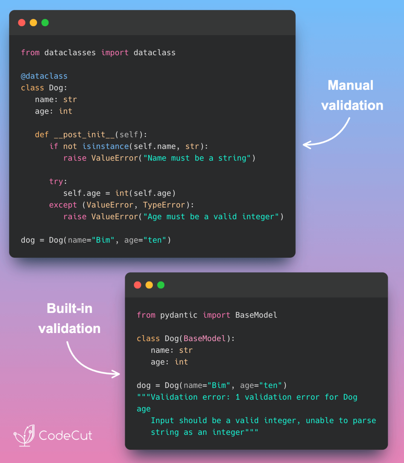
Dataclasses require manual implementation of validation logic. This means that you need to write custom code to validate the data, which can be time-consuming and error-prone.

Here’s an example of how you might implement validation using dataclasses:

from dataclasses import dataclass

@dataclass
class Dog:
name: str
age: int

def __post_init__(self):
if not isinstance(self.name, str):
raise ValueError("Name must be a string")

try:
self.age = int(self.age)
except (ValueError, TypeError):
raise ValueError("Age must be a valid integer, unable to parse string as an integer")

# Usage
try:
dog = Dog(name="Bim", age="ten")
except ValueError as e:
print(f"Validation error: {e}")

Validation error: Age must be a valid integer, unable to parse string as an integer

As you can see, implementing validation using dataclasses requires a significant amount of custom code.

Pydantic: Built-in Validation

Pydantic, on the other hand, offers built-in validation that automatically validates data and provides informative error messages. This makes Pydantic particularly useful when working with data from external sources.

Here’s an example of how you might define a Dog class using Pydantic:

from pydantic import BaseModel

class Dog(BaseModel):
name: str
age: int

try:
dog = Dog(name="Bim", age="ten")
except ValueError as e:
print(f"Validation error: {e}")

Validation error: 1 validation error for Dog
age
Input should be a valid integer, unable to parse string as an integer [type=int_parsing, input_value='ten', input_type=str]

As you can see, Pydantic automatically validates the data and provides a detailed error message when the validation fails.

Conclusion

While dataclasses require manual implementation of validation logic, Pydantic offers built-in validation that automatically validates data and provides informative error messages. This makes Pydantic a more convenient and efficient choice for working with data in Python, especially when working with data from external sources.

Link to Pydantic.

Favorite

Simplify Data Validation with Pydantic Read More »

Simplifying Repetitive Function Calls with partial in Python

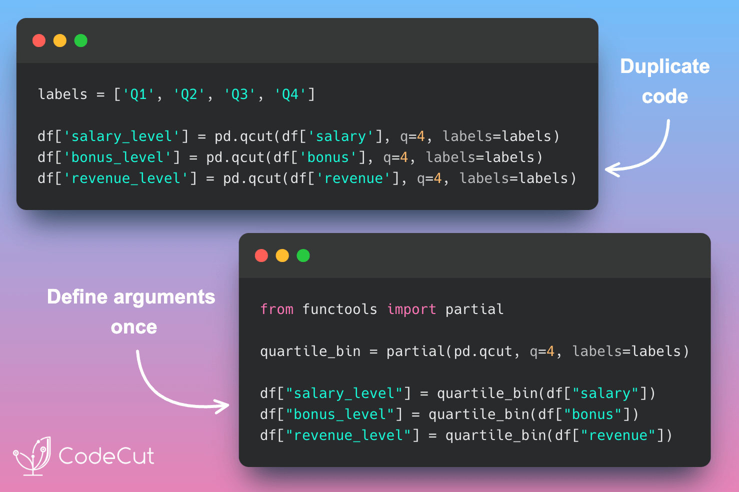
Repeatedly calling functions with some fixed arguments can lead to redundant code and reduced readability, causing unnecessary repetition throughout your codebase. In this article, we will explore how to simplify your code using functools.partial.

The Problem

Let’s consider an example where we have a DataFrame with salary, bonus, and revenue columns, and we want to perform quartile binning on each column.

import pandas as pd

df = pd.DataFrame({
'salary': [45000, 75000, 125000, 85000],
'bonus': [5000, 15000, 25000, 10000],
'revenue': [150000, 280000, 420000, 310000]
})

processed_df = df.copy()

# Repetitive binning operations
processed_df['salary_level'] = pd.qcut(processed_df['salary'], q=4, labels=['Q1', 'Q2', 'Q3', 'Q4'])
processed_df['bonus_level'] = pd.qcut(processed_df['bonus'], q=4, labels=['Q1', 'Q2', 'Q3', 'Q4'])
processed_df['revenue_level'] = pd.qcut(processed_df['revenue'], q=4, labels=['Q1', 'Q2', 'Q3', 'Q4'])
processed_df

salarybonusrevenuesalary_levelbonus_levelrevenue_level0450005000150000Q1Q1Q117500015000280000Q2Q3Q2212500025000420000Q4Q4Q438500010000310000Q3Q2Q3

This code is repetitive and hard to maintain. If we want to change the binning strategy, we have to modify it in multiple places.

The Solution

functools.partial is a higher-order function that allows us to create new function variations with pre-set arguments. We can use it to simplify our code and make it more maintainable.

from functools import partial

processed_df = df.copy()

# Create a standardized quartile binning function
quartile_bin = partial(pd.qcut, q=4, labels=["Q1", "Q2", "Q3", "Q4"])

# Apply the binning function consistently
processed_df["salary_level"] = quartile_bin(processed_df["salary"])
processed_df["bonus_level"] = quartile_bin(processed_df["bonus"])
processed_df["revenue_level"] = quartile_bin(processed_dfdf["revenue"])
processed_df

salarybonusrevenuesalary_levelbonus_levelrevenue_level0450005000150000Q1Q1Q117500015000280000Q2Q3Q2212500025000420000Q4Q4Q438500010000310000Q3Q2Q3

In this example, partial creates a standardized binning function with pre-set parameters for the number of quantiles and their labels. This ensures consistent binning across different columns.

Changing the Binning Strategy

If we need to change the binning strategy, we only need to modify it in one place.

processed_df = df.copy()

# Easy to create different binning strategies
quintile_bin = partial(pd.qcut, q=5, labels=["Bottom", "Low", "Mid", "High", "Top"])

processed_df["salary_level"] = quintile_bin(processed_df["salary"])
processed_df["bonus_level"] = quintile_bin(processed_df["bonus"])
processed_df["revenue_level"] = quintile_bin(processed_df["revenue"])
processed_df

salarybonusrevenuesalary_levelbonus_levelrevenue_level0450005000150000BottomBottomBottom17500015000280000LowHighLow212500025000420000TopTopTop38500010000310000HighLowHigh

By using functools.partial, we have simplified our code and made it more maintainable. We can easily create different binning strategies and apply them consistently across our DataFrame.
Favorite

Simplifying Repetitive Function Calls with partial in Python Read More »

Stop Writing Nested if-else: Use Python’s .get() Instead

The Problem with Multiple If-Else Statements

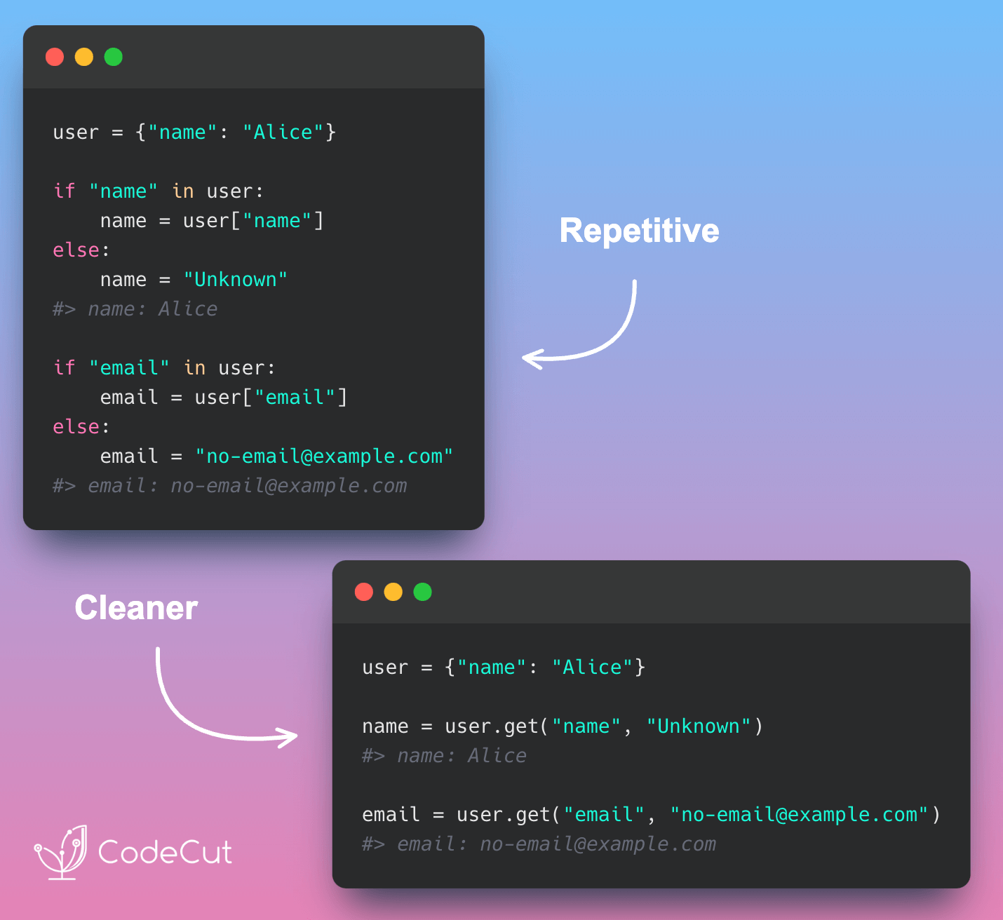
When working with Python dictionaries, you often need to access values that may not exist. The traditional approach of using multiple nested if-else statements can result in repetitive code that’s harder to maintain and more prone to errors.

Let’s consider an example where we have a dictionary user_data with keys “name”, “age”, and possibly “email”. We want to assign default values to these keys if they don’t exist.

# Checking dictionary values with multiple if-else
user_data = {"name": "Alice", "age": 30}

# Repetitive code with multiple default values
if "name" in user_data:
name = user_data["name"]
else:
name = "Unknown"

if "age" in user_data:
age = user_data["age"]
else:
age = 0

if "email" in user_data:
email = user_data["email"]
else:
email = "no-email@example.com"

print(f"{name=}")
print(f"{age=}")
print(f"{email=}")

Output:

name='Alice'
age=30
email='no-email@example.com'

As you can see, this approach is tedious and prone to errors.

A Cleaner Approach with the .get() Method

With the .get() method, we can access dictionary values with default values in a single line of code. This approach is not only more concise but also more readable and maintainable.

# Using .get() method for cleaner code
user_data = {"name": "Alice", "age": 30}

# Concise way to handle missing values
name = user_data.get("name", "Unknown")
age = user_data.get("age", 0)
email = user_data.get("email", "no-email@example.com")

print(f"{name=}")
print(f"{age=}")
print(f"{email=}")

Output:

name='Alice'
age=30
email='no-email@example.com'

Conclusion

In conclusion, the .get() method is a powerful tool for simplifying dictionary value access with default values. By using this method, you can write more concise, readable, and maintainable code.
Favorite

Stop Writing Nested if-else: Use Python’s .get() Instead Read More »

Debug Faster with Python 3.11’s Enhanced Tracebacks

Debugging code can be a tedious and time-consuming task, but having a clear traceback can greatly speed up the process. Python 3.11 introduces fine-grained error locations in tracebacks, allowing developers to quickly identify the exact location of errors.

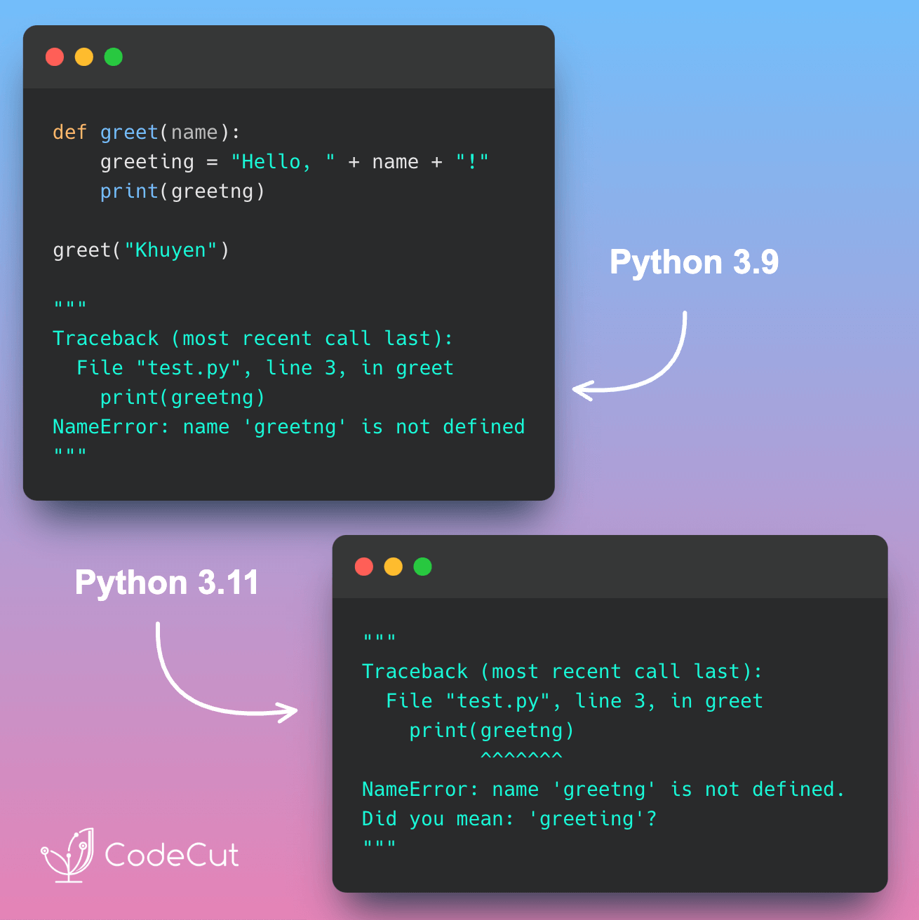
In this post, we’ll explore the difference in traceback between Python 3.9 and Python 3.11 using an example.

Example Code

Let’s consider the following Python code with a typo in the variable name:

def greet(name):
greeting = "Hello, " + name + "!"
print(greetng) # Error: Typo in variable name

greet("Khuyen")

Traceback in Python 3.9

When we run this code in Python 3.9, we get the following traceback:

Traceback (most recent call last):
File "/Users/khuyentran/book/Efficient_Python_tricks_and_tools_for_data_scientists/Chapter1/trackback_test.py", line 5, in <module>
greet("Khuyen")
File "/Users/khuyentran/book/Efficient_Python_tricks_and_tools_for_data_scientists/Chapter1/trackback_test.py", line 3, in greet
print(greetng) # Error: Typo in variable name
NameError: name 'greetng' is not defined

Traceback in Python 3.11

Now, let’s run the same code in Python 3.11:

Traceback (most recent call last):
File "/Users/khuyentran/book/Efficient_Python_tricks_and_tools_for_data_scientists/Chapter1/trackback_test.py", line 5, in <module>
greet("Khuyen")
File "/Users/khuyentran/book/Efficient_Python_tricks_and_tools_for_data_scientists/Chapter1/trackback_test.py", line 3, in greet
print(greetng) # Error: Typo in variable name
^^^^^^^
NameError: name 'greetng' is not defined. Did you mean: 'greeting'?

As you can see, Python 3.11 provides a more detailed traceback with fine-grained error locations. The ^^^^^^^ symbol points to the exact location of the error, making it easier to identify and fix the issue. Additionally, Python 3.11 suggests a possible correction, which can be helpful in cases where the error is due to a typo.
Favorite

Debug Faster with Python 3.11’s Enhanced Tracebacks Read More »

0
    0
    Your Cart
    Your cart is empty
    Scroll to Top

    Work with Khuyen Tran

    Work with Khuyen Tran