
Smoothing is useful for capturing the underlying pattern in time series data, especially for data with a strong trend or seasonal component.
The tsmoothie library is a fast and efficient Python tool for performing time-series smoothing operations.
To see how tsmoothie works, let’s generate a single random walk time series of length 200 using the sim_randomwalk() function.
import numpy as np
import matplotlib.pyplot as plt
from tsmoothie.utils_func import sim_randomwalk
from tsmoothie.smoother import LowessSmoother
# generate a random walk of length 200
np.random.seed(123)
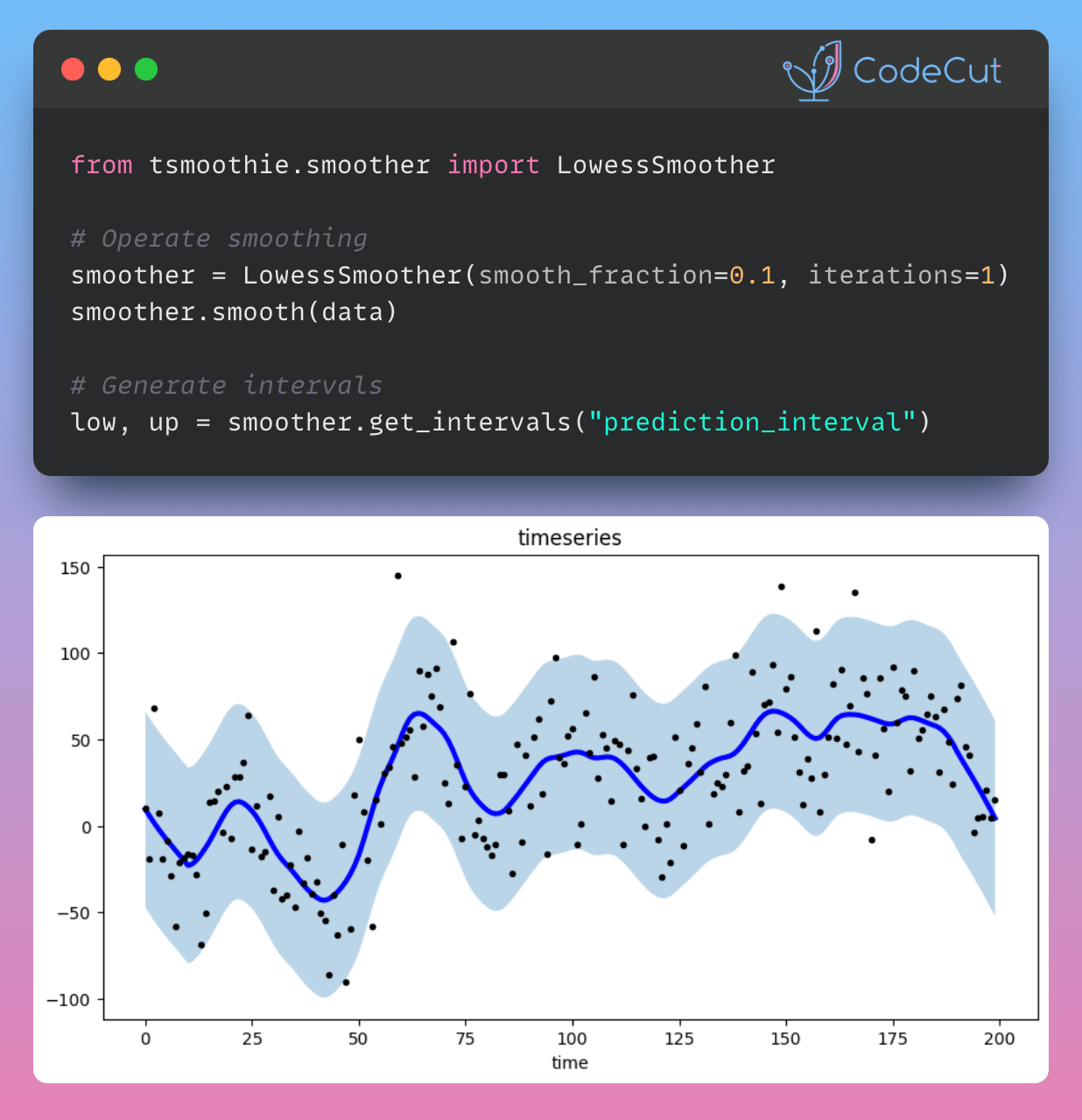
data = sim_randomwalk(n_series=1, timesteps=200, process_noise=10, measure_noise=30)Next, create a LowessSmoother object with a smooth_fraction of 0.1 (i.e., 10% of the data points are used for local regression) and 1 iteration. We then apply the smoothing operation to the data using the smooth() method.
# operate smoothing
smoother = LowessSmoother(smooth_fraction=0.1, iterations=1)
smoother.smooth(data)
After smoothing the data, we use the get_intervals() method of the LowessSmoother object to calculate the lower and upper bounds of the prediction interval for the smoothed time series.
# generate intervals
low, up = smoother.get_intervals("prediction_interval")
Finally, we plot the smoothed time series (as a blue line), and the prediction interval (as a shaded region) using matplotlib.
# plot the smoothed time series with intervals
plt.figure(figsize=(10, 5))

plt.plot(smoother.smooth_data[0], linewidth=3, color="blue")
plt.plot(smoother.data[0], ".k")
plt.title(f"timeseries")
plt.xlabel("time")

plt.fill_between(range(len(smoother.data[0])), low[0], up[0], alpha=0.3)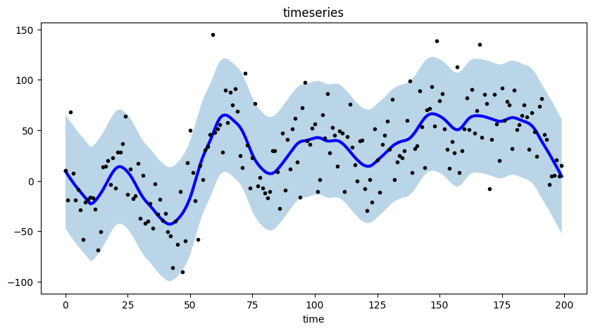
This graph effectively highlights the trend and seasonal components present in the time series data through the use of a smoothed representation.