
PySpark is a powerful tool for big data processing, but it lacks native support for time series data.
Tempo fills this gap with a more intuitive API, making it easier to perform common tasks like resampling and aggregating time-series data.
In this blog post, we’ll explore some examples that compare PySpark and Tempo, highlighting the benefits of using Tempo for time-series data analysis.
Data Preparation
Before we dive into the examples, let’s prepare our data. We’ll create a sample dataset of market data with the following columns:
symbol: the stock symbol (e.g. “AAPL” or “GOOGL”)event_ts: the timestamp of the event (e.g. “2024-01-01 09:30:00”)price: the current price of the stockvolume: the number of shares tradedbid: the current bid priceask: the current ask price
Here’s the code to create the sample dataset:
from pyspark.sql import functions as F
from pyspark.sql import Window

# Create sample market data
market_data = [
    ("AAPL", "2024-01-01 09:30:00", 180.50, 1000, 180.45, 180.55),
    ("AAPL", "2024-01-01 09:30:05", 180.52, 1200, 180.48, 180.58),
    ("AAPL", "2024-01-01 09:30:10", 180.48, 800, 180.45, 180.52),
    ("AAPL", "2024-01-01 09:30:15", 180.55, 1500, 180.50, 180.60),
    ("GOOGL", "2024-01-01 09:30:00", 140.25, 500, 140.20, 140.30),
    ("GOOGL", "2024-01-01 09:30:05", 140.30, 600, 140.25, 140.35),
    ("GOOGL", "2024-01-01 09:30:10", 140.28, 450, 140.25, 140.32),
    ("GOOGL", "2024-01-01 09:30:15", 140.32, 700, 140.28, 140.38),
]

# Create DataFrame
market_df = spark.createDataFrame(
    market_data, ["symbol", "event_ts", "price", "volume", "bid", "ask"]
)

# Convert timestamp string to timestamp type
market_df = market_df.withColumn("event_ts", F.to_timestamp("event_ts"))
Next, we’ll create a Tempo TSDF (Time Series DataFrame) from the market_df DataFrame. We’ll specify the event_ts column as the timestamp column and the partition column.
from tempo import *

# Create Tempo TSDF
market_tsdf = TSDF(market_df, ts_col="event_ts", partition_cols=["symbol"])
Now we’re ready to explore the examples!
Example 1: Get Data at Specific Time
Suppose we want to get the data at a specific time, say 2024-01-01 09:30:10. With PySpark, we would use the filter method to achieve this:
target_time = "2024-01-01 09:30:10"
pyspark_at_target = market_df.filter(F.col("event_ts") == target_time)
pyspark_at_target.show()
With Tempo, we can use the at method to achieve the same result:
tempo_at_target = market_tsdf.at(target_time)
tempo_at_target.show()
Both methods produce the same output:
+------+-------------------+------+------+------+------+
|symbol|           event_ts| price|volume|   bid|   ask|
+------+-------------------+------+------+------+------+
|  AAPL|2024-01-01 09:30:10|180.48|   800|180.45|180.52|
| GOOGL|2024-01-01 09:30:10|140.28|   450|140.25|140.32|
+------+-------------------+------+------+------+------+
Example 2: Get Data between Time Interval
Suppose we want to get the data between a time interval, say 2024-01-01 09:30:05 and 2024-01-01 09:30:15. With PySpark, we would use the filter method with a conditional statement:
start_ts = "2024-01-01 09:30:05"
end_ts = "2024-01-01 09:30:15"
pyspark_interval = market_df.filter(
    (F.col("event_ts") >= start_ts) & (F.col("event_ts") <= end_ts)
)
pyspark_interval.show()
With Tempo, we can use the between method to achieve the same result:
tempo_interval = market_tsdf.between(start_ts, end_ts)
tempo_interval.show()
Both methods produce the same output:
+------+-------------------+------+------+------+------+
|symbol| event_ts| price|volume| bid| ask|
+------+-------------------+------+------+------+------+
| AAPL|2024-01-01 09:30:05|180.52| 1200|180.48|180.58|
| AAPL|2024-01-01 09:30:10|180.48| 800|180.45|180.52|
| AAPL|2024-01-01 09:30:15|180.55| 1500| 180.5| 180.6|
| GOOGL|2024-01-01 09:30:05| 140.3| 600|140.25|140.35|
| GOOGL|2024-01-01 09:30:10|140.28| 450|140.25|140.32|
| GOOGL|2024-01-01 09:30:15|140.32| 700|140.28|140.38|
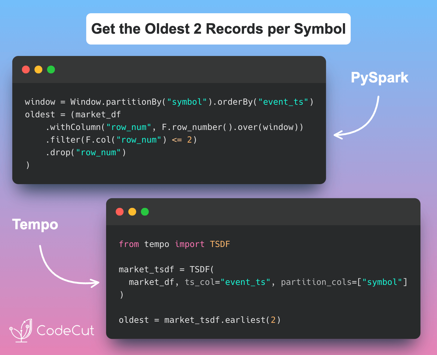
+------+-------------------+------+------+------+------+Example 3: Get the Oldest N Records per Symbol
Suppose we want to get the oldest N records per symbol, say N=2. With PySpark, we would use the row_number function with a window specification:
n = 2
windowSpec = Window.partitionBy("symbol").orderBy("event_ts")
pyspark_oldest = (
    market_df.withColumn("row_num", F.row_number().over(windowSpec))
    .filter(F.col("row_num") <= n)
    .drop("row_num")
)
pyspark_oldest.show()
With Tempo, we can use the earliest method to achieve the same result:
tempo_oldest = market_tsdf.earliest(n)
tempo_oldest.show()
Both methods produce the same output:
+------+-------------------+------+------+------+------+
|symbol|           event_ts| price|volume|   bid|   ask|
+------+-------------------+------+------+------+------+
|  AAPL|2024-01-01 09:30:00| 180.5|  1000|180.45|180.55|
|  AAPL|2024-01-01 09:30:05|180.52|  1200|180.48|180.58|
| GOOGL|2024-01-01 09:30:00|140.25|   500| 140.2| 140.3|
| GOOGL|2024-01-01 09:30:05| 140.3|   600|140.25|140.35|
+------+-------------------+------+------+------+------+
Example 4: Moving Averages
Suppose we want to calculate the moving average of the price column with a 10-second window. With PySpark, we would use the avg function with a window specification:
market_df = market_df.withColumn("event_ts_seconds", F.unix_timestamp("event_ts"))
movingWindowSpec = (
    Window.partitionBy("symbol").orderBy("event_ts_seconds").rangeBetween(-10, 0)
)

pyspark_moving_stats = market_df.withColumn(
    "mean_price", F.avg("price").over(movingWindowSpec)
)

pyspark_moving_stats.select("symbol", "event_ts", "price", "mean_price").show()
With Tempo, we can use the withRangeStats method to achieve the same result:
tempo_moving_stats = market_tsdf.withRangeStats("price", rangeBackWindowSecs=10)
tempo_moving_stats.select("symbol", "event_ts", "price", "mean_price").show()
Both methods produce the same output:
+------+-------------------+------+------------------+
|symbol|           event_ts| price|        mean_price|
+------+-------------------+------+------------------+
|  AAPL|2024-01-01 09:30:00| 180.5|             180.5|
|  AAPL|2024-01-01 09:30:05|180.52|            180.51|
|  AAPL|2024-01-01 09:30:10|180.48|             180.5|
|  AAPL|2024-01-01 09:30:15|180.55|180.51666666666665|
| GOOGL|2024-01-01 09:30:00|140.25|            140.25|
| GOOGL|2024-01-01 09:30:05| 140.3|           140.275|
| GOOGL|2024-01-01 09:30:10|140.28|140.27666666666667|
| GOOGL|2024-01-01 09:30:15|140.32|             140.3|
+------+-------------------+------+------------------+
Example 5: Grouped Statistics
Suppose we want to calculate the mean, min, and max of the price column grouped by symbol and a 5-second window. With PySpark, we would use the groupBy method with a window specification:
pyspark_grouped = market_df.groupBy("symbol", F.window("event_ts", "5 seconds")).agg(
    F.avg("price").alias("mean_price"),
    F.min("price").alias("min_price"),
    F.max("price").alias("max_price"),
)
pyspark_grouped.show()
Output:
+------+--------------------+----------+---------+---------+
|symbol|              window|mean_price|min_price|max_price|
+------+--------------------+----------+---------+---------+
|  AAPL|{2024-01-01 09:30...|     180.5|    180.5|    180.5|
|  AAPL|{2024-01-01 09:30...|    180.52|   180.52|   180.52|
|  AAPL|{2024-01-01 09:30...|    180.48|   180.48|   180.48|
|  AAPL|{2024-01-01 09:30...|    180.55|   180.55|   180.55|
| GOOGL|{2024-01-01 09:30...|    140.25|   140.25|   140.25|
| GOOGL|{2024-01-01 09:30...|     140.3|    140.3|    140.3|
| GOOGL|{2024-01-01 09:30...|    140.28|   140.28|   140.28|
| GOOGL|{2024-01-01 09:30...|    140.32|   140.32|   140.32|
+------+--------------------+----------+---------+---------+
With Tempo, we can use the withGroupedStats method to achieve the same result:
tempo_grouped = market_tsdf.withGroupedStats(
    metricCols=["price"], freq="5 seconds"
)
tempo_grouped.show()
Output:
+------+-------------------+----------+---------+---------+
|symbol|           event_ts|mean_price|min_price|max_price|
+------+-------------------+----------+---------+---------+
|  AAPL|2024-01-01 09:30:00|     180.5|    180.5|    180.5|
|  AAPL|2024-01-01 09:30:05|    180.52|   180.52|   180.52|
|  AAPL|2024-01-01 09:30:10|    180.48|   180.48|   180.48|
|  AAPL|2024-01-01 09:30:15|    180.55|   180.55|   180.55|
| GOOGL|2024-01-01 09:30:00|    140.25|   140.25|   140.25|
| GOOGL|2024-01-01 09:30:05|     140.3|    140.3|    140.3|
| GOOGL|2024-01-01 09:30:10|    140.28|   140.28|   140.28|
| GOOGL|2024-01-01 09:30:15|    140.32|   140.32|   140.32|
+------+-------------------+----------+---------+---------+
Tempo provides a more intuitive and concise API for working with time-series data, making it easier to perform common tasks like resampling and aggregating time-series data.